FUNDAMENTALS OF ENZYME STRUCTURE AND KINETICS IN BIOLOGICAL SYSTEMS - O. A. Naumenko - 2017

2 General Issues in the Kinetics and Thermodynamics of Enzymatic Reactions

2.1 Laws of Classical Thermodynamics in Biochemistry

Over the past 30 years, enzymatic kinetics has experienced rapid development. Enzymatic kinetics investigates how the Rate of Enzymatic reactions changes depending on Enzyme Concentration, Substrate Concentration, the presence of activators and inhibitors, fluctuations in Temperature and medium pH, as well as the mechanisms regulating enzyme activity during a reaction.

2.1.1 Basic Concepts of Kinetics and Thermodynamics. Thermodynamic Systems

Kinetics is a branch of physics that studies Changes in the parameters of a thermodynamic system during various thermodynamic processes.

Enzymatic kinetics explores the Laws of Thermodynamics, specifically heat and energy exchanges in biological systems. Living biological systems can achieve a dynamic or stationary state (dynamic equilibrium) when The amount of matter and energy entering the system equals the amount leaving it.

Enzymatic kinetics examines the mechanism, energetics, regulation, and conformational changes of Enzymes during enzymatic reactions. Energy transformations in biological systems are studied by a branch of biochemistry known as bioenergetics.

Chemical thermodynamics applies the laws of thermodynamics to thermodynamic systems. The collection of bodies participating in a reaction is called a thermodynamic system (TS), while bodies outside the system are referred to as the external environment. Thermodynamic systems are classified into open and closed. The laws of thermodynamics are strictly applicable only to closed systems.

Closed systems exchange only energy, but not mass, with their surroundings. Open systems are capable of exchanging both mass and energy with their environment and, under certain conditions, can achieve dynamic equilibrium or a stationary state, though not thermodynamic equilibrium with maximum Entropy.

Biological organisms are open thermodynamic systems that exchange both energy and matter with their environment.

Thermodynamically balanced systems exhibit no macroscopic changes. Their internal energy is minimal, and they exist in a state of complete disorder. Living systems achieve thermodynamic equilibrium only after death.

All open systems, together with their surroundings, form a closed system.

When heat exchange occurs and at least partial diffusion is possible between the bodies comprising the system, a thermodynamic system is formed. A thermodynamic system can interact with its surroundings, and this interaction is detected via Heat transfer or the performance of work.

If all interaction between the System and Its environment is completely absent, the system is referred to as isolated.

If the state of a thermodynamic system remains unchanged and this stability is not caused by any external stationary process, the system is said to be in equilibrium. A system consisting of a single phase is homogeneous; otherwise, it is heterogeneous.

The laws of thermodynamics apply to closed systems. Therefore, for research and calculations in bioenergetics, METABOLISM/2.html">THE CONCEPT OF an isolated system (characterized by minimal energy exchange) has been introduced.

Thermodynamic systems can be classified according to their aggregate properties. The properties of a thermodynamic system are referred to as its thermodynamic parameters.

Extensive properties, such as weight and volume, are proportional to mass. Intensive properties, such as temperature and pressure, are independent of mass. The state of a system in equilibrium can be described by the combination of its intensive properties. Thermodynamic parameters describe only the Current state of a system, disregarding its history. Consequently, The change in parameters when a system transitions from one state to another is independent of the reaction pathway and is determined solely by the Thermodynamic parameters of the initial and final states.

Mass (M) and volume (V) are universally accepted terms. Pressure (P) characterizes the interaction with the external environment, measured as force per unit of surface area.

Temperature (T), which is determined by the intensity of the thermal motion of the molecules making up the system, is not a simple concept; it encompasses the notion of heat differences. Heat transfer occurs between bodies of different temperatures, leading to temperature equalization. The absolute temperature scale is based on The Second Law of thermodynamics, with its origin at absolute zero (- 273.16° K).

At absolute zero, the portion of any substance's energy that depends on temperature (thermal energy) is zero, although the energy of the particles constituting the substance does not, of course, vanish at zero temperature.

2.1.2 Thermodynamic Process

Any modification in the parameters of a thermodynamic system that results in a change to at least one thermodynamic parameter is called a thermodynamic process (TP).

Characteristics of a reversible thermodynamic process. If a system passes through equilibrium states during a thermodynamic process, the work performed by the system itself under given conditions will be maximal, while the work performed on the system will be minimal; such a process is referred to as a reversible TP.

Conversely, a thermodynamic process occurring under some limited impact on the system is defined as a non-equilibrium thermodynamic process. The work done by such a system is less than the maximum work in a reversible process.

If the sole result of the reverse process in an isolated system is the return of the system from its final state to the initial one, such a process is called a reversible thermodynamic process.

If As a result of a direct or reverse reaction in the system or its surroundings, prolonged changes in the thermodynamic parameters of the system take place, the thermodynamic process is called irreversible.

The reason for irreversibility is that processes in thermodynamic systems proceed through non-equilibrium states. Thermodynamic parameters are unambiguous only for reversible processes when the system is in equilibrium at any given moment and in every part of it. If a system is taken out of a state of stable equilibrium, a thermodynamic process arises that opposes the external influence (Le Chatelier–Braun principle).

2.1.3 First Law of Thermodynamics

The First Law of thermodynamics states that energy in a thermodynamic system cannot be created from nothing nor destroyed, but can only be transformed from one form into another. This means that the energy content (U) in a thermodynamic system increases when the thermodynamic system performs work (A) or heat is transferred (Q):

∆U = А + Q

где ∆U - изменение энергии ТС; А - работа ТС; Q - теплота ТС.

В случае ТП, когда изменение энергии системы ∆U = 0,

А = - Q (2.2)

Отсюда проистекает невозможность создания вечного двигателя первого рода.

Если над ТС не совершается никакой работы, т. е. ∆U = ∆Q, то при равновесном давлении (∆Р = 0) для объема V можно определить новую функцию:

H = U + PV (3.3)

где Н - энтальпия (или теплосодержание ТС); U - внутренняя энергия ТС; Р - давление в ТС; V - объем ТС.

Закон Гесса: теплота превращения в ТС не зависит от пути протекания ТП.

При экзотермическом процессе - выделенная ТС теплота считается отрицательной величиной (теплосодержание системы уменьшается), т. к. положительным условно считается тепло, полученное ТС (+Н)- это эндотермический процесс, сопровождающийся увеличением теплосодержания ТС. Протекающие в живых организмах анаболические процессы представляют собой эндотермические реакции, а катаболические - экзотермические.

2.1.4 Второй закон термодинамики

Все процессы в природе протекают в одном направлении, т. е. они необратимы. Необратимость в термодинамике означает, что ТП процесс не может идти в ТС в обратном направлении без изменения энтропии. Энтропия выражается следующим уравнением:

∆S = ∆Q / Т, (3.4)

где ∆S - изменение энтальпии ТС; ∆Q - изменение теплоты ТС; Т - Температура ТС.

Дифференциальное изменение энтропии равняется отношению элементарного количества теплоты к абсолютной температуре. Основываясь на втором законе термодинамике, все природные процессы, не противоречащие первому закону термодинамики, можно разделить на две группы:

- самопроизвольные ТП при данных условиях;

- не самопроизвольные ТП.

Невозможна реакция, дающая только перенос тепла от тела с более низкой температурой к телу с более высокой температурой. Это означает, что работа в ТС не может быть выполнена исключительно за счет тепловой энергии окружающей среды, другими словами, невозможно создание вечного двигателя второго рода.

При обратимых ТП в изолированной ТС энтропия остается неизменной, при необратимых процессах она возрастает. Если в результате необратимого процесса изолированная система приходит в равновесие, то ее энтропия достигает максимума. Следовательно, изменение энтропии определяет направление ТП и одновременно условия термодинамического равновесия.

THE PRINCIPLE OF constancy or increase of entropy holds true only for an isolated system. In an isolated system, the increase in entropy serves as a measure of the irreversibility of a process. Living organisms maintain their internal order (constant entropy) by acquiring additional energy from the environment in the form of nutrients (chemical energy) or sunlight (electromagnetic energy), and they return an equivalent amount of energy to the environment in another form, predominantly as heat, which dissipates throughout the

rest of the universe. Living organisms must continuously increase their entropy to maintain internal order.

2.1.5 Characteristic Functions of Thermodynamic Systems

A characteristic function is a state function of a thermodynamic system by means of which its properties can be expressed. A potential is defined as a function whose change is related to the work done by the system. In thermodynamics, the following characteristic functions are most widely used:

1) isochoric-isothermal potential of the system — Helmholtz energy (∆F);

2) isobaric-isothermal potential of the system — Gibbs energy (∆G);

3) internal energy of the system (∆U);

4) enthalpy of the system (∆Н);

5) entropy of the system (∆S).

The internal energy (∆U) of the system is determined According to the equation:

∆U = T∆S - Р∆V (2.5)

where ∆U is the change in internal energy of the system; T is temperature; ∆S is entropy; Р is pressure; ∆V is volume.

Enthalpy ∆Н is the change in the heat content of a system at constant pressure and entropy.

∆Н = T∆S + V∆P, (2.6)

where ∆Н is the change in heat content or enthalpy of the system; T is temperature; ∆S is entropy; ∆Р is pressure; V is volume.

Entropy ∆S is a measure of the disorder of a system, defined as the quantity of heat supplied to the system at a constant temperature.

∆S = ∆Q / Т, (2.7)

where ∆S is the change in entropy of the system; T is temperature; ∆S is entropy; ∆Q is the change in heat.

Helmholtz energy is the Free energy of a system available to perform useful work at constant volume and temperature (isochoric-isothermal potential).

F = U - TS, (2.8)

where F is the free energy of the system; T is temperature; ∆S is entropy; U is the internal energy of the system.

Gibbs energy is the free energy of a system available to perform useful work at constant pressure and temperature (isobaric-isothermal potential).

G = H — TS (2.9)

where G is the Gibbs energy; T is temperature; S is entropy; Н is enthalpy.

Review Questions for the Topic

1. What does enzyme kinetics study?

2. WHAT IS A thermodynamic process and what are its types?

3. Define a thermodynamic system.

4. What types of thermodynamic systems exist?

5. What is an open thermodynamic system?

6. State the first law of thermodynamics.

7. State the second law of thermodynamics.

8. Thermodynamic process and its types.

9. Enthalpy and entropy.

10. Characteristic functions in thermodynamics.

2.2 Michaelis-Menten Kinetics

2.2.1 Chemical kinetics. The concept of reaction order

Chemical kinetics is the branch of science concerned with chemical processes, their mechanisms, and laws governing their progression over time.

Chemical kinetics studies The rate of a chemical reaction taking into account various conditions: reactant concentrations, temperature, ambient pH, and the presence or absence of catalysts.

In chemistry, one mole of a substance corresponds to one molecule of that substance, and the amount of substance in moles is denoted by the stoichiometric coefficient. According to the law of mass action, the reaction order is determined by the sum of the powers of the reactant concentrations.

For example, in the course of a chemical reaction, 1 mole of substance A is converted into 1 mole of substance B: 1 mole A —> 1 mole B

This is a unimolecular reaction, or a first-order reaction.

If, during the reaction, 1 mole of substance A reacts with 1 mole of substance B to form 1 mole of substance C: A + B —> C, then this reaction is referred to as a bimolecular or second-order reaction.

2.2.2 Michaelis-Menten Kinetics

In 1835, Jöns Jacob Berzelius first suggested that reactions in Living organisms are driven by a "new force" which he termed "catalytic". Berzelius formulated the principle of catalysis, including among catalytic agents the enzyme diastase, which catalyzed the Hydrolysis of Starch faster than sulfuric acid.

Preliminary Experiments on the Kinetics of Enzymatic reactions showed that the rate of an enzymatic reaction described by the equation: E + S —> E + P does not depend on the enzyme and substrate concentrations in the same way as a conventional second-order chemical reaction.

The earliest attempt to mathematically describe enzymatic reactions was undertaken by Duclaux in 1898. Brown (1902) and, independently, Henri (1903) first hypothesized The formation of an enzyme-substrate complex during the reaction.

In 1913, Michaelis and Menten published their theory on the general Mechanism of Enzymatic reactions. Their equation became a foundational principle for all kinetic studies of enzymes.

Thus, Michaelis and Menten hypothesized that The Mechanism of a typical two-stage enzymatic reaction is described by the scheme:

Class="center"> (2.10),

where: E is the enzyme; S is the substrate; ES is the enzyme-substrate complex; P is the enzymatic reaction product; k₁ is the dissociation constant of The First stage (second-order reaction);

k₂ is the dissociation constant of the Second Stage of enzyme-substrate complex breakdown (first-order reaction).

In this scheme, k₁ = k_s, where k_s is the dissociation constant of the enzyme-substrate complex, and the rate of the enzymatic reaction is determined by the rate of breakdown of the enzyme-substrate complex into the product, i.e., the rate of the second stage:

v₀ = k₂ [ES], (2.11)

where: k₂ is the dissociation constant of the second stage of enzyme-substrate complex breakdown (first-order reaction); v₀ is the initial rate of the enzymatic reaction; [ES] is the concentration of the enzyme-substrate complex.

The model assumes that the equilibrium of the first stage of the enzymatic reaction between the free enzyme, substrate, and enzyme-substrate complex is established rapidly compared to the overall rate of the enzymatic reaction (rapidly establishing equilibrium of the first stage, k₂ « k₁, k_-1). In this case, the second stage of the reaction has virtually no effect on the rate of the first stage; therefore, the dissociation constant of the enzyme-substrate complex K_s can be used to express the enzyme concentration.

(2.12)

where K_s is the dissociation constant of the enzyme-substrate complex; [E] is the enzyme concentration; [S] is the substrate concentration; [ES] is the concentration of the enzyme-substrate complex.

The total enzyme concentration in the reaction mixture is expressed by the material balance equation for the enzyme:

[E]₀=[E] + [ES] = [ES] (K_s/[S]+1), (2.13)

where [E]₀ is the initial enzyme concentration; K_s is the dissociation constant of the enzyme-substrate complex; [E] is the enzyme concentration; [S] is the substrate concentration;

[ES] is the concentration of the enzyme-substrate complex.

Then the concentration of the enzyme-substrate complex is:

(2.14)

The reaction reaches its maximum velocity when all of the enzyme is in the form of the enzyme-substrate complex:

V_max=k_s[ES]=k_s[E]₀, (2.15)

where V_max is the maximum rate of the enzymatic reaction; k_s is the dissociation constant of the enzyme-substrate complex; [E]₀ is the initial enzyme concentration; [S] is the substrate concentration; [ES] is the concentration of the enzyme-substrate complex.

This condition is met if the reaction proceeds at an excess substrate concentration: [S]₀>> [E]₀. From the previous equations, we obtain:

(2.16)

where v₀ is the initial rate of the enzymatic reaction; V_max is the maximum rate of the enzymatic reaction; K_s is the dissociation constant of the enzyme-substrate complex; [S] is the substrate concentration.

This is the classical Michaelis-Menten Equation, which is still used today to describe The kinetics of enzymatic reactions, and the value of the Michaelis constant under these conditions, K_m = K_s, represents a measure of the enzyme's affinity for the substrate. The maximum rate of the enzymatic reaction is achieved when the concentration of the enzyme-substrate complex is numerically equal to the total enzyme concentration (i.e., when all the enzyme is bound to the substrate in the complex).

In this case, the dependence of the enzymatic reaction rate on the concentration (E) largely depends on The ratio of enzyme and substrate concentrations. If the substrate concentration reaches a maximum and significantly exceeds the enzyme concentration ([S] » [E]), then the rate of the enzymatic reaction increases linearly and is directly proportional to the enzyme concentration—that is, the higher the concentration [E], the higher the reaction rate will be.

2.2.3 Limitations of Michaelis-Menten Kinetics

Michaelis and Menten derived the equation taking into account two conditions: a rapidly established equilibrium of the first stage and a significant excess of substrate. It was later proven that the equation is valid when seven conditions or postulates are met.

Postulates for the validity of the Michaelis-Menten equation:

1) a kinetically stable enzyme-substrate complex is formed during the reaction, which persists at a certain concentration for a specific period;

2) the constant $K_s$ determined using the equation is the dissociation constant of the enzyme-substrate complex: this holds true only if $k_2 \ll k_1, k_{-1}$;

3) the substrate concentration remains unchanged throughout the reaction, i.e., [S] = [S]₀;

4) the reaction product rapidly dissociates from the enzyme, meaning the reaction proceeds in two stages;

5) the second stage of the reaction is irreversible. Since this is practically unattainable, we consider only the initial rates of enzymatic reactions;

6) exactly one substrate molecule binds to each Active Site of the enzyme;

7) for all reacting species, concentrations can be used instead of activities.

2.2.4 Formation of a Kinetically Stable Enzyme-Substrate Complex (Justification of the First Postulate)

To date, X-ray crystallography data provide hundreds of pieces of experimental evidence demonstrating the formation of kinetically stable enzyme-substrate complexes during enzymatic reactions. Although other theories have also been proposed, enzymatic reactions can proceed without the formation of an enzyme-substrate complex.

1. The Theory of telekinetic interactions suggests that the enzyme increases the energy of the substrate molecule via certain telekinetic interactions (electrostatic attraction or repulsion, electromagnetic radiation, etc.).

2. The theory of elastic collisions. It is postulated that the enzyme transfers energy to the substrate through elastic collisions. In this process, the substrate molecule attains an energy exceeding a certain threshold and can either enter a reaction or decompose to form products.

Despite the fact that kinetic equations were formulated for these theories under conditions where the enzyme is separated from the substrate by a solvent (i.e., telekinesis in energy transfer to the substrate could theoretically occur), such theories have not yet found experimental confirmation.

This implies that the formation of a kinetically stable enzyme-substrate complex invariably occurs in all known enzymatic reactions. Therefore, the first condition defining the validity of Michaelis-Menten kinetics can be considered proven.

2.3 Nature of the Constant K in the Michaelis-Menten Equation

2.3.1 Briggs-Haldane Steady-State Kinetics (Justification of the Second Postulate)

The second postulate states that the constant $K_s$ in equation (2.16) is the dissociation constant of the enzyme-substrate complex.

In 1925, Briggs and Haldane proved that the original Michaelis-Menten equation is valid only under the condition $k_2 \ll k_1, k_{-1}$, i.e., when the equilibrium of the first stage (E + S ⇄ ES) is established very rapidly compared to the rate at which the equilibrium of the second stage is established.

Therefore, such kinetic mechanisms that obey the initial Michaelis-Menten condition and feature a single rate-limiting step, relative to which equilibria in all other steps are established rapidly, are referred to as "rapid equilibrium" systems.

If $k_2$ is comparable in magnitude to $k_{-1}$, Briggs-Haldane kinetics or steady-state kinetics is applied: where the amount

of the formed enzyme-substrate complex equals the amount of the dissociated complex. In this case, the equation for the initial rate of the enzymatic reaction will be as follows:

(2.17)

Where $V$ is the rate of the enzymatic reaction; $V_{max}$ is the maximum reaction velocity; $K_m$ is the Michaelis constant; [S] is the substrate concentration; [E] is the enzyme concentration; $K_1$ is the dissociation constant of the first stage (second-order reaction);

This equation is similar to equation (2.16), but it broadens the scope and applicability of the original Michaelis-Menten equation.

2.3.2 Nature of the Constant K in the Michaelis-Menten Equation

If an enzymatic reaction satisfies the condition of rapidly established equilibrium in the first stage and $k_2 \ll k_1, k_{-1}$, then the dissociation constant $K$, determined by investigating the dependence of the reaction rate on substrate concentration, corresponds to the dissociation constant of the enzyme-substrate complex (the first stage) $K_s$.

Under the stationarity condition: k₂ = k1 (Briggs-Haldane kinetics), the constant found by the same method will be the Michaelis constant, where K_м= (к_-1 + к₂)/ к₁.

In other reactions, when k₁ «k₂, the Michaelis constant equals k₂/k₁ and is referred to, according to Van Slyke, as the kinetic constant K_s.

When reaction conditions change, the value of the constant K may also vary. For instance, in the case of peroxidase at a high concentration of the proton-donor substrate, this constant acts as a kinetic constant (K_k). As the concentration of the proton-donor substrate decreases, the constant turns into the Michaelis constant – K_m, and at very low levels of the proton-donor substrate, we obtain the dissociation constant of the enzyme-substrate complex – K_s.

Since the value of the Michaelis constant varies depending on reaction conditions, K_m is also denoted as apparent K_m (K_m(app)). According to equation (2.16), the plot of the enzymatic reaction rate versus the initial substrate concentration S has a hyperbolic shape (Figure 2.1). This graph shows that at the beginning of the reaction, the reaction rate increases directly and linearly with increasing substrate concentration. The reaction order in this case is first-order. The reaction rate in this section reaches its maximum (V_max) when all the substrate is bound to the enzyme, and the enzymatic reaction constant corresponds to K_s.

Figure 2.1 - Plot of enzymatic reaction rate versus substrate concentration S.

Further on, as the substrate concentration increases, the curve changes from a straight line to a parabola. In this case, the reaction order becomes fractional (n = 1/2). In this part of the reaction, S is consumed, its concentration decreases and becomes [S] = K_m, while the reaction rate is equal to 1/2 of V_max. With a further increase in substrate concentration S, the reaction rate does not increase, the reaction order becomes zero (n = 0), and the reaction rate V = const.

Thus, the physical meaning of the Michaelis constant (K_m) is that it represents the substrate concentration [S] at which the enzymatic reaction rate is equal to 1/2 of the maximum rate.

The value of constants for each enzymatic reaction is determined experimentally, and their magnitude depends on the pH of the medium, temperature, and the presence of an inhibitor (activator). If V_max and K_m are determined for an enzyme, one can calculate the optimal concentration of substrate S.

2.3.3 Methods for Graphical Determination of Kinetic Parameters

For practical tasks in enzymology, the hyperbolic plot of the enzymatic reaction rate versus substrate concentration S is quite inconvenient. Therefore, linearization methods for experimental data are used in practice.

The Lineweaver-Burk coordinates (1/V and 1/S) and Dixon-Eisenthal coordinates (1/V and [S]) are most frequently used to determine the kinetic parameters of enzymatic reactions.

The Lineweaver-Burk method is known as the double-reciprocal plot method. The graph showing the dependence of the enzymatic reaction rate on substrate concentration is linear and presented in Figure 2.2.

Figure 2.2 - Lineweaver-Burk plot of enzymatic reaction rate versus substrate concentration S.

The reciprocal values (1/V) of the enzymatic reaction rate in Lineweaver-Burk coordinates are calculated using formula 2.18:

(2.18)

where V is the enzymatic reaction rate; V_max is the maximum enzymatic reaction rate; K_m is the Michaelis constant; [S] is the substrate concentration.

Review Questions on the Topic

1. Reaction order and methods for its determination.

2. History of The Development of enzyme kinetics.

3. The Michaelis-Menten equation.

4. Limitations of Michaelis-Menten kinetics.

5. Formation of a kinetically stable enzyme-substrate complex.

6. The Nature of the constant K in the Michaelis-Menten equations.

7. What is the physical Significance of the Michaelis constant?

8. What is the shape of the plot of enzymatic reaction rate versus substrate concentration according to the Michaelis-Menten equation?

9. What are the axes in the Lineweaver-Burk plot?

10. What is a kinetic constant?

11. What evidence exists for the first postulate?

2.4 Kinetic analysis of two-stage enzymatic reactions that do not obey the Michaelis-Menten equation

The third postulate of enzyme kinetics states that the substrate concentration does not change during the reaction, i.e., [S]_t = [S]₀. This implies the presence of a sufficiently large excess of substrate. However, in many cases, this condition is not met. On the one hand, a large excess of substrate is not used in "in vitro" reactions with certain enzymes due to frequent substrate inhibition of the enzyme's catalytic activity. An excess of substrate is also typically not achieved "in vivo".

In enzymatic reactions where the substrate is not in excess and, consequently, its concentration changes over time during the course of the reaction, the dissociation constant takes the form:

(2.19)

where Ks is the dissociation constant of the enzyme-substrate complex; [S]₀ is the initial substrate concentration; [ES] is the concentration of the enzyme-substrate complex;

[E]₀ is the enzyme concentration at THE START OF the reaction; [P] is the concentration of the enzymatic reaction product.

The initial reaction rate will then be:

(2.20)

where V_max is the maximum rate of the enzymatic reaction; Ks is the dissociation constant of the enzyme-substrate complex; [S]_t is the substrate concentration at a given time point.

2.4.1 Variation of substrate concentration during an enzymatic reaction (justification of the third postulate)

Equation (2.20) can be solved using two different sets of conditions for the enzymatic reaction, where [S]₀ ≠ [S]_t:

1) if this inequality holds due to large values of t, i.e., when more than 5% of the initial substrate concentration is consumed during the reaction (at the start of the reaction, the condition of substrate excess was met);

2) if the enzyme concentration cannot be neglected compared to the substrate concentration and, therefore, the concentration of the enzyme-substrate complex must be taken into account (the reaction time is short, but the condition of substrate excess was not initially met).

2.4.1.1 Solution for the first case: If t is large and [ES] « [S]₀, equation (2.20) transforms into the following:

(2.21)

where Ks is the dissociation constant of the enzyme-substrate complex; [S]₀ is the initial substrate concentration; [ES] is the concentration of the enzyme-substrate complex;

[E]₀ is the enzyme concentration at the start of the reaction; [P] is the concentration of the enzymatic reaction product.

For the substrate concentration [S]_t, which changes during the reaction, a satisfactory approximation is given by the value ([S]₀+[S]_t)/2. Then the average rate can be expressed as:

(2.22)

where V_max is the maximum rate of the enzymatic reaction; K_m is the Michaelis constant; [S]₀ is the initial substrate concentration; [S]_t is the substrate concentration at a given time point.

2.4.1.2 Solution for the second case. When the condition of substrate excess is not initially met, but substrate consumption does not exceed 5%. In this case, the product concentration [P] can be neglected, but the concentration of the enzyme-substrate complex [ES] must be taken into account,

(2.23)

where Ks is the dissociation constant of the enzyme-substrate complex; [ES] is the concentration of the enzyme-substrate complex; [E] is the enzyme concentration;

The quadratic equation with respect to the substrate concentration:

(2.24)

where Ks is the dissociation constant of the enzyme-substrate complex; [S]₀ is the initial substrate concentration; [S] is the substrate concentration;

a is a coefficient defined as:

а = Ks+[E]₀ - [S]₀, (2.25)

where Ks is the dissociation constant of the enzyme-substrate complex; [S]₀ is the initial substrate concentration; [S] is the substrate concentration.

The solution to this quadratic equation is

(2.26)

where Ks is the dissociation constant of the enzyme-substrate complex; [S]₀ is the initial substrate concentration; [S] is the substrate concentration; a is a coefficient.

(2.27)

Then the reaction rate V can be expressed by the equation

(2.28)

where k₂ is the rate constant of the second step; [S]₀ is the initial substrate concentration; [ES] is the concentration of the enzyme-substrate complex; [Е]₀ is the initial enzyme concentration; V_max is the maximum enzymatic reaction rate.

Expressing λ from the last equation, we obtain

(2.29)

where V is the enzymatic reaction rate; V_max is the maximum enzymatic reaction rate.

A comparison of the values calculated by this method with those obtained from the exact integrated Michaelis-Menten equation shows that the error in determining Km is only 1% and 4% at 30% and 50% substrate consumption, respectively. Consequently, these equations can be used to calculate the kinetic parameters of enzymatic reactions over extended reaction times and significant substrate depletion.

2.4.2 Procedure for determining kinetic constants under the condition [S]₀ ≠ [S]_t

The procedure for determining the constants in this case is as follows.

1. In preliminary experiments (under substrate excess conditions), V_max is determined;

2. Under the conditions where [E]₀~[S]₀, the reaction rates are measured at various substrate concentrations;

3. Using equation (2.29), the parameter λ is calculated for each determined rate;

4. Using the calculated values of λ, we determine K_s.

From the intersection point of this line with the abscissa axis, we find K_s, where the slope of the line equals 1/[Е]₀. Thus, studying how the enzymatic reaction rate depends on the substrate concentration under the condition [E]₀~[S]₀ allows us to determine the absolute concentration of the enzyme's active sites.

Review Questions

1. What does the third postulate of enzyme kinetics state?

2. The approximate solution of the Michaelis-Menten equation for long reaction times.

3. What are the conditions for the first variant of the approximate solution to the Michaelis-Menten equation?

4. What are the conditions for the second variant of the approximate solution to the Michaelis-Menten equation?

5. What is the methodology for finding kinetic constants under the condition [S]₀ ≠ [S]_t?

2.5 Effect of Reversible Effectors on Enzyme Kinetics

2.5.1 Mechanisms of Reversible Effector Action on Enzyme Kinetics

Substances that alter the catalytic activity of an enzyme are called effectors.

The interaction between an enzyme and an effector is a chemical reaction and can therefore be fully reversible, partially reversible, or practically irreversible. If the inhibition process is irreversible, the kinetic reaction does not obey the Michaelis-Menten mechanism, which is based on the equilibrium between the free and bound forms of the enzyme.

In the case of reversible inhibitors, the Michaelis-Menten equation can be used to describe the enzyme kinetics. Depending on how inhibitors affect the kinetic parameters of the enzymatic reaction, they are classified as follows:

a) Competitive Inhibitors — substances in the presence of which K_m increases while V_max remains unchanged. The effect caused by such inhibitors can be partially or completely reversed by increasing the substrate concentration. An example is the reversible competitive inhibition of the enzyme succinate dehydrogenase by malonic acid, where succinic acid serves as the substrate (Figure 2.3);

Figure 2.3 — Reversible competitive inhibition of succinate dehydrogenase by malonic acid

b) non-competitive inhibitors — substances that inactivate the enzyme or the enzyme-substrate complex by decreasing V_max without affecting K_m. In this case, increasing the substrate concentration does not lead to an increase in the reaction rate. Non-competitive inhibitors include heavy Metal Ions that reversibly react with the -SH groups of cysteines.

Many competitive inhibitors are structurally similar to substrates. Such inhibitors are referred to as substrate analogs.

Non-competitive inhibitors bind to the allosteric site of the enzyme.

2.5.2 Kinetics of Enzymatic reactions involving an Effector

In the general case, The Effect of a reversible effector on a two-stage enzymatic reaction can be represented by the following scheme:

(2.30)

where E is the enzyme; S is the substrate; P is the reaction product; k_s is the dissociation constant of the enzyme-substrate complex; k₂ is the dissociation constant of the second stage;

k_E is the dissociation constant of the enzyme-effector complex; EE is the enzyme-effector complex; EES is the ternary effector-enzyme-substrate complex.

For the initial rate of an enzymatic reaction (under the condition [S]₀, [E]₀>> [E]₀, where [E] is the effector concentration, α is a coefficient indicating the factor by which the rate of the first stage changes in the presence of the effector, and β is a coefficient representing the change in the rate of the second stage under the steady-state equilibria of the First and Second Stages of the enzymatic reaction), the following holds true:

(2.31)

where [S]₀ is the initial substrate concentration; [ES] is the concentration of the enzyme-substrate complex; [Е]₀ is the initial enzyme concentration; [Э] is the effector concentration; K_s is the dissociation constant of the enzyme-substrate complex; к₂ is the second-stage dissociation constant; кэ is the dissociation constant of the enzyme-effector complex; а is the rate change coefficient for the first stage; β is the rate change coefficient for the second stage.

Depending on the numerical values of α and β, the effector can act either as an inhibitor or as an activator of the enzymatic reaction. The following types of inhibition are distinguished:

- complete competitive inhibition;

- complete non-competitive inhibition;

- uncompetitive inhibition;

- simple activation;

- mixed inhibition;

- mixed activation.

2.5.2.1 Complete competitive inhibition (α —> ∞, β has no defined meaning), the rate of the enzymatic catalytic reaction is described by the equation:

(2.32)

where [S]₀ is the initial substrate concentration; [Е]₀ is the initial enzyme concentration; [I] is the inhibitor concentration; к_s is the dissociation constant of the enzyme-substrate complex; к₂ is the second-stage dissociation constant; ki is the dissociation constant of the enzyme-inhibitor complex.

The Lineweaver-Burk plot appears as a family of lines intersecting on the ordinate axis (Figure 2.4).

Figure 2.4 - Plot of the relationship under complete competitive inhibition

By plotting experimental data in coordinates (К_М(_Каж), [I]), the competitive inhibition constant Ki can be determined using formula 2.33:

(2.33)

where Км is the Michaelis constant; [I] is the inhibitor concentration; к_s is the dissociation constant of the enzyme-substrate complex; ki is the dissociation constant of the enzyme-inhibitor complex.

2.5.2.2 Complete non-competitive inhibition (α —> 1, β =0). In this case, the rate of the enzymatic catalytic reaction is given by the equation:

(2.34)

where [S]₀ is the initial substrate concentration; [Е]₀ is the initial enzyme concentration; [I] is the inhibitor concentration; к_s is the dissociation constant of the enzyme-substrate complex; к₂ is the second-stage dissociation constant; ki is the dissociation constant of the enzyme-inhibitor complex.

The Lineweaver-Burk plot appears as a family of lines intersecting on the abscissa axis (Figure 2.5).

Figure 2.5 - Plot of the relationship under complete non-competitive inhibition

By presenting experimental data in coordinates (1/k_kat, [I]), the non-competitive inhibition constant K can be determined knowing the value of к_к:

(2.35)

where k_к is the catalytic constant; [I] is the inhibitor concentration; k₂ is the dissociation constant of the second stage; кi is the enzyme-inhibitor complex dissociation constant.

2.5.2.3 Uncompetitive inhibition (α = β ≤ 1). In this case, the rate of the enzymatic reaction is:

(2.36)

where [S]₀ is the initial substrate concentration; [Е]₀ is the initial enzyme concentration; [I] is the inhibitor concentration; к_s is the enzyme-substrate complex dissociation constant; к₂ is the dissociation constant of the second stage; кi is the inhibition constant; α is the coefficient of variation for the first-stage rate; β is the coefficient of variation for the second-stage rate.

The values of the catalytic constant k_kat and the apparent Michaelis constant К_М(каж) of the enzymatic reaction decrease to the same extent with an increase in effector concentration; therefore, the plots in

Lineweaver-Burk coordinates take the form of a family of parallel lines (Figure 2.6).

Figure 2.6 - Plot for uncompetitive inhibition. For equation analysis, the expression for the catalytic constant

(2.37)

where к_к is the catalytic constant; [I] is the inhibitor concentration; к₂ is the dissociation constant of the second stage; кi is the inhibition constant; α is the coefficient of variation for the first-stage rate, which is conveniently rearranged into the following form:

(2.38)

where к_к is the catalytic constant; [I] is the inhibitor concentration; к₂ is the dissociation constant of the second stage; кi is the inhibition constant; α is the coefficient of variation for the first-stage rate.

From the plot constructed in coordinates (1/(k_kat/k_{2 -1}), 1/[I]), the values of α and Кi can be determined separately.

2.5.2.4 Non-competitive activation (α = 1, β >1). In this case, the substrate and activator bind independently to the active site, forming a ternary complex (enzyme-substrate-activator), which leads to an increase in the rate of product formation in the enzymatic reaction. Therefore, the initial rate of the enzymatic reaction is given by:

(2.39)

where [S]₀ is the initial substrate concentration; [Е]₀ is the initial enzyme concentration; [А] is the activator concentration; к_s is the enzyme-substrate complex dissociation constant; к₂ is the dissociation constant of the second stage; к_А is the activation constant; β is the coefficient of variation for the second-stage rate.

The dependence in Lineweaver-Burk coordinates appears as a pencil of lines intersecting on the abscissa axis.

2.5.2.5 Mixed types of inhibition and activation (α ≠ 1, β ≠ 1). In the case of mixed inhibition or activation, the Lineweaver-Burk plots form a pencil of lines corresponding to various effector concentrations, which intersect at a common point in the upper right, upper left, or lower left quadrant depending on the values of α and β (Figure 2.7).

Figure 2.7 - Plots for mixed-type inhibition

The coordinates of the intersection point of the line bundle are determined by the values of the constants α and β.

Review questions for the topic

1. What are the possible modes of interaction between an enzyme and an effector?

2. What is meant by reversible inhibition?

3. What does irreversible inhibition signify?

4. What does competitive activation signify?

5. What do the coefficients α and β denote?

6. What will the rate dependence plot look like in the case of mixed inhibition?

7. What will the rate dependence plot look like in non-competitive activation?

8. What will the rate dependence plot look like in uncompetitive inhibition?

9. What will the rate dependence plot look like in full non-competitive inhibition?

10. What will the rate dependence plot look like in full competitive inhibition?

2.6 Substrate Excess Inhibition and Activation

2.6.1 MECHANISMS OF SUBSTRATE Inhibition

It has been established for many enzymes that upon The addition of excess substrate, the rate of the catalyzed reaction neither increases further nor remains constant at concentrations above saturation, but instead decreases; that is, inhibition develops. This phenomenon has been termed substrate excess inhibition.

Regarding its mechanisms, five Different types of inhibition can be proposed:

1) the substrate binds to the enzyme via two or more groups, and only a substrate molecule bound in this manner can participate in the reaction. If A large number of substrate molecules are present, a situation may arise where one substrate molecule binds to one binding site of the enzyme, while another substrate molecule binds to a different site instead of interacting with the second group of the first substrate molecule. Since only a molecule bound to the enzyme at two points can participate in the reaction, the enzyme molecule holding two substrate molecules will be inactive, i.e., inhibition will occur;

2) at high concentrations, the substrate can bind to a secondary site distinct from the active center of the protein. In this case, it can ''non-competitively'' inhibit the rate of breakdown of the substrate bound at the active site;

3) the enzyme requires the presence of a specific activator to exhibit activity. If the substrate is capable of forming a complex with the activator, an excess of substrate depletes the activator, thereby decreasing enzyme activity;

4) for Reactions Involving Two or more substrates, an excess of one substrate is capable of binding to the binding site of the other, thereby inhibiting the reaction;

5) increasing the substrate concentration above a certain threshold non-specifically inhibits the reaction due to an increase in Ionic strength.

2.6.2 Kinetic Analysis of Enzyme-Catalyzed Reactions under Substrate Inhibition

For many enzymes, the dependence of v on [S]₀ can be quantitatively described based on the assumption that an enzymatically inactive ternary complex ES₂ is formed:

(2.39)

where E is the enzyme; S is the substrate; P is the reaction product; ES is the enzyme-substrate complex; ES₂ is the ternary enzyme-substrate complex; K_s' is the dissociation constant of the ternary enzyme-substrate complex; k₂ is the dissociation constant of the second step.

In this case, the rate equation for the enzymatic reaction takes the form:

(2.40)

where [S]₀ is the initial substrate concentration; [E]₀ is the total enzyme concentration at the start of the reaction; K_s is the dissociation constant of the enzyme-substrate complex;

k₂ is the dissociation constant of the second step.

The Analysis of the equation is divided into two parts:

1) at low substrate concentrations ([S]₀₂«K_s'), equation (2.40) simplifies to the classic Michaelis-Menten equation (no substrate inhibition is observed). By plotting the data in Lineweaver-Burk coordinates, we find к₂ and K_s;

2) at high substrate concentrations ([S]₀» K_s), equation (2.40) takes the form:

(2.41)

where v is the enzyme-catalyzed reaction rate; [S]₀ is the initial substrate concentration; [Е]₀ is the enzyme concentration at the beginning of the reaction; K_s is the dissociation constant of the enzyme-substrate complex; K_s' is the dissociation constant of the ternary enzyme-substrate complex; к₂ is the dissociation constant of the second step.

Equation (2.41) can be rewritten as:

(2.42)

and by plotting 1/v versus [S]0, the values of к₂ and K_s' can be determined. If the values of к₂ found in both concentration ranges coincide, it means that scheme (2.39) is applicable for the formal Description of the kinetics of the studied enzymatic reaction.

In the second model, the ternary complex ES₂ retains catalytic activity, but it is lower compared to the enzyme-substrate complex ES (β<1).

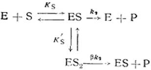(2.43)

where E is the enzyme; S is the substrate; P is the reaction product; ES is the enzyme-substrate complex; ES₂ is the ternary enzyme-substrate complex; β is the coefficient of rate change for the second step; K_s' is the dissociation constant of the ternary enzyme-substrate complex; к₂ is the dissociation constant of the second step.

In this case, the rate of the enzymatic reaction under steady-state conditions and [S]₀» [Е]₀ is described by the equation:

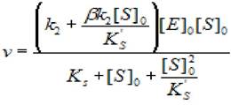(2.44)

where v is the enzyme-catalyzed reaction rate; [S]₀ is the initial substrate concentration; [Е]₀ is the enzyme concentration at the beginning of the reaction; K_s is the dissociation constant of the enzyme-substrate complex; K_s' is the dissociation constant of the ternary enzyme-substrate complex; β is the coefficient of rate change for the second step; к₂ is the dissociation constant of the second step.

The analysis of the scheme is also divided into two regions. At low substrate concentrations, к₂ and K_s are determined. At high concentrations, the equation simplifies to the following relationship:

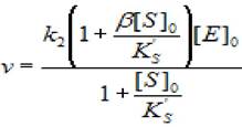(2.45)

where v is the enzyme-catalyzed reaction rate; [S]₀ is the initial substrate concentration; [Е]₀ is the enzyme concentration at the beginning of the reaction; K_s is the dissociation constant of the enzyme-substrate complex; K_s' is the dissociation constant of the ternary enzyme-substrate complex; β is the coefficient of rate change for the second step; к₂ is the dissociation constant of the second step.

By plotting the graph in coordinates (1/(1 -к_эфф/к₂), 1/[S]₀) for high substrate concentrations, we find the values of β and K_s'.

The third type of substrate inhibition occurs when multiple substrate molecules bind to the enzyme-substrate complex, converting it into an inactive state.

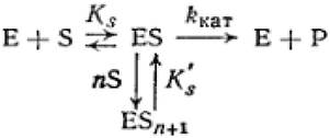(2.46)

where E is the enzyme; S is the substrate; P is the reaction product; ES is the enzyme-substrate complex; ES_n+2 is the enzyme-substrate complex bound with 2 or more molecules; n is the number of substrate molecules bound to the enzyme; K_s' is the dissociation constant of the ternary enzyme-substrate complex; к_кат is the catalytic constant or the dissociation constant of the second step.

To analyze such cases, a graphical method has been developed that allows determining the number of substrate molecules in the inactive enzyme-substrate complex. The Processing of experimental data in these cases is carried out as follows:

1) from the plot in coordinates (v, lg[S]₀) we determine [S]_opt;

2) for various n using formula (83) we find the product K_SK_S';

3) for each n, we plot a graph in coordinates (1/[S]₀ + [S]oⁿK_sK_s', 1/v). The value of n at which the plot is linear corresponds to relationship (2.44), and consequently, to model (2.45) with the found value of n.

We have examined 3 possible schemes of Enzyme Inhibition caused by substrate excess. To determine the appropriate inhibition mechanism, one must first plot the experimentally obtained velocity values in the coordinates (v, lg[S]₀).

The symmetrical shape of the resulting bell-shaped curve indicates the absence of enzymatic activity in the SES complex (Figure 2.8).

Figure 2.8 - Coordinate plot for all models of substrate inhibition

If the right branch of the graph (at high substrate concentrations) is gentler compared to the left branch, this points to the enzymatic activity

of a ternary complex (0 <β <1). Conversely, if the substrate inhibits enzyme activity, the right side of the graph will be steeper.

2.6.2 Substrate Activation

In certain cases, as the substrate concentration increases, the rate of the enzymatic reaction exceeds the theoretical maximum velocity of the enzymatic reaction calculated from data obtained at low substrate concentrations. The simplest model of such activation corresponds to a scheme where β>1. Experimental Data analysis is performed similarly (2.43). The only difference is that it is more convenient to plot the graph in the coordinates (1/(к_эфф/к_2-1), 1/[S]₀) according to the equation:

(2.47)

where [S]₀ is the initial substrate concentration; K_s is the dissociation constant of the enzyme-substrate complex; K_s' is the dissociation constant of the ternary enzyme-substrate complex; β is the coefficient of rate change in the second stage; к₂ is the dissociation constant of the second stage.

Review Questions on the Topic

1. What are the possible modes of interaction between an enzyme and excess substrate?

2. Write the reaction scheme for substrate excess inhibition resulting in the formation of a substrate-enzyme-substrate ternary complex.

3. How is the velocity of the enzymatic reaction determined in this case?

4. Write the reaction scheme for substrate activation.

5. How can the kinetic parameters of the enzymatic reaction be determined in this case?

2.7 Factors Affecting Enzymatic Activity. Effect of pH and Temperature on Enzyme Kinetics

2.7.1 Factors Affecting Enzymatic Activity

The catalytic activity of enzymes is influenced by numerous factors that can alter their Structure or chemical nature. These factors include:

1) pH;

2) temperature;

3) fluid forces (hydrodynamic forces, hydrostatic pressure, and surface tension);

4) chemical agents (alcohol, urea, or hydrogen peroxide);

5) irradiation (light, sound, ionizing radiation).

Sometimes the decrease in catalytic activity caused, for instance, by a pH change is reversible. In such cases, returning to initial conditions restores the enzyme's activity. In a sense, this situation is analogous to the aforementioned case of reversible inhibition. Minor fluctuations in any of the above factors only slightly shift the equilibrium (or quasi-stationary state) characteristic of a given enzymatic reaction. In general, deviation from the conditions typical of the native enzyme's biological environment must be relatively small (or short-term). Otherwise, the probability of Enzyme inactivation increases.

2.7.2 Reversible Effect of temperature on Enzyme Catalytic Activity

The boundary between "reversible" and "irreversible" protein inactivation is not always clearly defined. For example, an enzyme subjected to brief heating can fully recover its activity upon cooling to its characteristic "operating" temperature. On the other hand, a more prolonged heating at the same temperature, or an equally brief heat Treatment at a higher temperature, may result in only partial recovery of enzyme activity upon subsequent cooling. This behavior of enzyme Proteins becomes understandable when considering the relationship between their Structure and function, The impact of Molecular Dynamics on protein function, and the potential disruption of certain weak bonds within the native Cell/13.html">Protein Structure due to changing environmental conditions.

At high temperatures, when The process of thermal enzyme inactivation begins to dominate, the dependence of reaction rate on temperature is disrupted.

Thus, enzymatic reactions exhibit a bell-shaped dependence of reaction rate on temperature. This is explained by the superimposition of two effects: an increase in reaction rate with rising temperature, and the acceleration of thermal Denaturation of the protein molecule, which leads to enzyme inactivation at elevated temperatures. Denaturation of most proteins begins in the temperature range of 45° C to 50° C and completes very rapidly at 55° C.

2.7.3 Effect of pH on the Kinetics of Enzymatic Reactions in Solutions

Enzymes, like all proteins, are composed of Amino Acids. Depending on the pH, the side chains of Certain amino acids—and consequently the protein as a whole—can acquire a charge. Charged groups are frequently constituents of enzyme active sites, since A number of Enzymatic Catalysis mechanisms are based on

Acid-Base Catalysis. A prerequisite for acid-base catalysis can be the presence of a specific charge on the ionizable groups of the active site. It follows that the catalytically active form of the enzyme exists in only one strictly defined ionization state, and depending on the pH, a larger or smaller fraction of the total enzyme present in the mixture can convert into this form (Figure 2.9).

Figure 2.9 - Dependence of enzyme activity on pH

At pH values significantly differing from the optimum, the Forces Stabilizing the conformation of the native enzyme protein are disrupted, which can lead to its denaturation—the loss of tertiary conformation and, consequently, catalytic activity. In this case, even after restoring the optimal pH, enzyme renaturation remains unlikely.

Review Questions for the Topic Studied

1. What factors affect enzymatic activity?

2. The effect of pH on the kinetics of enzymatic reactions in solutions.

3. How does the rate of enzymatic reactions change with temperature variation?

4. What processes occur in the Enzyme Structure during denaturation?

5. What is renaturation?