BOTANY VOLUME 4 - ECOLOGY - 2007

12. BASICS OF PLANT ECOLOGY

12.5. Ecosystem and Its Structure

An ecosystem is defined as a complex of interacting abiotic and biotic components within a specific bounded area. The abiotic matrix (habitat) is referred to as the biotope, while the living component constitutes the biocenosis. This heavily simplified scheme separates what is inherently inseparable, as the biocenosis continuously modifies and shapes the biotope; even its initial establishment creates its characteristic living space (biotope), since a completely abiotic state does not exist in nature. Spruce forests do not initially grow on typical forest soils; rather, such soils develop where spruces have grown for a sufficiently long time. Nevertheless, the biotope-biocenosis dichotomy symbolizes the changes in Physical and Chemical conditions alongside the organisms associated with them.

12.5.1. Structure OF THE Biocenosis

12.5.1.1. Hierarchical Structure

A biocenosis is the assemblage of All living organisms within an ecosystem: plants, animals, Fungi, and microorganisms. The assemblage of all plants is termed a phytocenosis, or plant community. Each species within such an "association" (phytosociology, see ch. 14) is typically represented by numerous individuals, collectively referred to as a population (a reproducing association). A population encompasses all age stages of a species, as well as individuals present latently in the soil as seeds. A population consists of genetically distinct individuals or genetically distinct groups of individuals that originated clonally (genetically identical within the clone)—known as ramets. Thus, an individual Organism embodies a specific genotype or, in the case of a genetically identical individual ramet, a part of a genet (synonymous with a clone). Because individuals originating from seeds can also be genetically identical (apomixis, see 10.1.3.3), clones containing genetically uniform individuals occur more frequently than might be assumed from their Morphology alone (e.g., the apomictic species Taraxacum officinale). A comparable hierarchical structure is also found in communities of animals, fungi, and microorganisms.

12.5.1.2. Taxonomic Structure

The character of an ecosystem is shaped by the presence of specific plant species. These serve as indicators of local environmental conditions, which is why a species list is frequently established at the onset of ecosystem analysis (indicator species, see 12.5.2.2; indicator value, see 14.3.3). Determining the number of species and the relative Abundance (frequency) of individual species represents an essential biological inventory, designated in the phytosociology (see 14.3.3) of German-speaking countries as community structure (Bestandesstruktur). Because the English term "structure" is almost exclusively used to denote Spatial Structure (see 12.5.1.5), it is more appropriate to apply METABOLISM/2.html">THE CONCEPT OF "species composition" here. The term biodiversity is commonly used to quantitatively assess species richness. However, it also encompasses intraspecific genetic diversity and supra-specific levels, namely the variety of plant communities (see 14.2.4.1).

12.5.1.3. Functional Structure

All photosynthetically active organisms are grouped under the term primary producers. They are contrasted by consumers (which feed on living organisms) and decomposers (reducers that break down organic matter). Consumers function directly as herbivores (phytophages feeding on plants) or indirectly as predators (of the first, second, or third order). Dead organic remains are ultimately decomposed by A wide variety of decomposers. These notably include detritivores (detritus being dead litter; litter-feeding mites and earthworms) and mineralizers (Bacteria and specialized fungi). Such food chains, or preferably food webs, interlink the members of every ecosystem, just as energy flows and nutrient cycles do. These connections can feature feedback loops, enabling a limited degree of self-regulation directed against external changes (Fig. 12.4).

Class="center">Fig. 12.4. Ecosystem concept. Simplified scheme of a complete ecosystem, i.e., a broad self-regulating structure of interactions between living organisms and their environment (for explanations, see text)

Within a plant community, one can distinguish functional groups, or functional types. Theoretically, there are as many of these as there are species (see Introduction to ch. 12); if functionally vastly different age stages of a single individual are considered (e.g., seedling vs. tree), their number even exceeds that of species. The concept of functional groups aims to reduce the often immense species diversity into a small number of categories with "similar functioning," which is primarily necessary for ecosystem modeling and theoretical generalizations. Numerous attempts at such grouping exist; some important ones are outlined here. The simplest and perhaps most widely used is grouping by morphotypes (grasses, shrubs, trees, or rosette-forming graminoids vs. deep-rooting vs. shallow-rooting forms, etc.) and phenotypes (annuals, perennials, summer-green, evergreen, etc.; phenology, see 7.7 and 12.3.1). Grouping by physiotypes is based on metabolic characteristics, such as photosynthetic pathways: C₃, C₄, or CAM types (see 6.5.7 – 6.5.9), light requirements corresponding to their position in the community (shade and sun plants), substrate specialization (calciphiles and calcifuges), or resistance properties (to drought, soil salinity, frost, heat). Symbiotypes are based on the capacity for Symbiosis with nitrogen-fixing bacteria or specialized mycorrhizal fungi. Further criteria for group formation can include

various Other forms of mutualism and parasitism.

A concept originally inspired by zoology is grouping according to dominant life strategies, which became a classical division of plants based on their lifestyle into r-strategists (where 'r' highlights reproductive capacity, emphasizing their resilience) and K-strategists (where 'K' highlights competitive ability, emphasizing their predominantly vegetative mode of reproduction); over time, many different plant strategy concepts have been developed. Particularly well known is Grime's triangle system, or CSR strategists (Competitors, Stress-tolerators, Ruderals). It is derived from a two-dimensional matrix in which plants are grouped according to their tolerance to stress and disturbance (low or high); one of the four combinations (high stress and high disturbance) is considered non-existent, leaving three categories. These mark the extreme situations at the corners of the triangle. Every plant occupies a specific position between these extremes. The distances from the corner points are termed radii; for instance, the stress radius indicates the degree of stress tolerance of a species. Like every attempt to typify The Diversity of life situations, this concept has also been criticized as overly simplistic.

P. Grubb, by contrast, argues that the category of stress-tolerant plants should be subdivided into three distinct strategies, as their behavior can change over the course of their lifetime. He distinguishes between species that maintain their strategy type throughout life from seedling to adult (low-flexibility strategy), species that tolerate stress well only at the seedling stage (switching strategy), and finally species that can reorganize and to some extent change their type, transitioning to another category when conditions become highly favorable (gearing strategy). Indicators of stress tolerance include, among others, slow growth, perennial Organs, low reproductive effort, and relatively thick leaves with low nitrogen content.

The list of Examples of typification and grouping could be continued at length. Experience has shown that functional groups often exhibit the expected common Functions only to a very limited extent, and species-specific differences within functional groups are frequently greater than those between the groups themselves. Furthermore, individuals of different ages within a species may be assigned to different functional groups, complicating species-grouping efforts. Depending on the objectives, different grouping Methods are preferred or even newly devised groups are created (e.g., groups of species resistant to ozone, heavy metals, or waterlogging). Morphotypes and phenotypes may still represent the most practical functional groups for a non-taxonomic description of phytocenological structure.

12.5.1.4. Material Structure

International rules have been established for the naming and categorization of plant substance within an ecosystem (all data without exception are given in dry weight after drying at 80 – 100 °C). The living, above-ground and below-ground plant component of an ecosystem is termed plant biomass. Biomass also includes dead internal Tissues (lignified structures) that nevertheless belong to the living plant. External dead plant parts (above- and below-ground) are designated as necromass (standing dead). The aggregate of all living and dead external plant parts is called phytomass. This is contrasted with detached dead plant parts within the ecosystem—litter—with a distinction made between surface litter (lying on the soil surface) and subterranean litter (e.g., dead roots). Organic residues in which organ structures can no longer be recognized with the naked eye are classified under the humus complex (soil organic matter, SOM), which encompasses all transitions from raw humus to the complex of humic acid molecules within the organic fraction of the soil. The organic substance of animal origin (mostly small soil fauna) and microorganisms is very minor (<0.1%) and is usually added to the soil carbon pool or ignored altogether, which, of course, does not diminish the vital function of these organisms in the ecosystem.

12.5.1.5. Spatial Structure

The mode of occupation of aerial space and soil determines not only the general outward appearance but also The properties of an ecosystem. The morphology of shoots and roots of dominant plant species, particularly community geometry or architecture, gives each ecosystem its unique identity and determines where energy conversion takes place and from where Water and nutrients are drawn. The most important parameters of above-ground structure are the height of dominants, leaf area index, and the vertical distribution of leaf area; for below-ground structure, they include ROOT system types, maximum rooting depth, and the vertical distribution of roots in the soil profile.

The Leaf Area Index (LAI) is a dimensionless unit indicating how many square meters of leaf surface are present per 1 m² of ground surface (actual leaf surface regardless of its spatial orientation; for thick or non-flat leaves, this corresponds to their maximum projected area). In closed plant communities on well-developed soils with adequate water supply, LAI values reach 5 – 8. For most cultivated crops, the maximum LAI reaches nearly 4. Leaf Area Density (LAD), measured in inverse meters (m^-1), is given for the community as a whole by dividing the LAI by the community height or the height of individual strata (The ratio of leaf surface area in m² to 1 m³ of community volume). LAI and LAD determine the light profile within the community (see 13.1.3).

The majority of fine roots are typically located close to the soil surface (<1 m), often even in the upper 20 cm of the soil profile, where most mineralizers and mycorrhizal fungi are also concentrated. A portion of the root systems may reach considerable depths (see Table 13.3). Such deep-rooting systems primarily serve to secure water supply. The stratified distribution of individual species' roots in the soil profile is a classic example of niche differentiation, which significantly drives biodiversity. Deep roots may also function to moisten upper soil horizons (hydraulic lift, see 13.6.4). The diversity of root system types frequently surpasses the diversity of SHOOT types and constitutes an essential structural feature of every ecosystem.

12.5.2. Biotope: Habitat and Environmental Factors

12.5.2.1. Habitat and Locality

Habitat factors (at a given time under fixed local conditions) comprise climate, relief, soil, and the biotic influences of other organisms present (e.g., shading forest trees). These are countered by environmental factors, which act directly and fluctuate strongly over short periods: actual solar radiation, warmth, humidity, Chemical factors, as well as mechanical and biological disturbances. Plants respond to these factors through growth, development, structural features, and resistance (Fig. 12.5).

Fig. 12.5. Habitat and environmental factors. The secondary habitat factors manifested in a locality represent a complex of primary habitat and environmental factors that act directly on various plant structures and processes. They exert a mutual influence. Furthermore, a variety of feedback loops can be established between the plant and its environment

A habitat is understood as an area characterized by uniform factors. The term "locality" refers to the specific place where a plant actually grows (= Location). The actual living conditions of localities within the same habitat can vary significantly due to microclimate, local microrelief, and soil properties, as well as neighbouring plant species and animals. It is well established that localities are not random; plant species naturally occur in similar localities where they feel "at home," which refers to their natural habitat (habitat). Natural habitat is a relatively narrow concept applied to a specific plant species or group of species, whereas habitat is a broader concept focused on local conditions regardless of which species grow there. Plant species may also inhabit several Different types of natural environments. These three concepts are often confused or used as synonyms; there is no single unambiguous English Translation for the Russian word "местообитание" (the laconic "site" is mostly used).

12.5.2.2. Climate and Microclimate

Climate is defined as the multi-year average state of the atmosphere and the mean course of meteorological conditions. Weather refers to the atmospheric situation observed at a given moment. The diverse climates of the Earth are primarily determined by the quantity and seasonal distribution of heat and precipitation. These differences can be clearly illustrated using climadiagrams (Fig. 12.6).

Fig. 12.6. Climadiagrams: A — for a warm-temperate climate with continental influence, winter rains, and summer droughts; B — for a temperate climate with oceanic influence, with precipitation throughout the year; C — for a humid tropical climate with a distinct rainy season and a (relatively) dry season. Air temperatures shown are measured in the shade at a height of 2 m. Abscissa: months; ordinate: one graduation = 10 °С and correspondingly 20 mm of precipitation. a — station (location); b — altitude above sea level; c — number of observation years; d — mean annual Temperature, °С; e — mean annual precipitation, f — mean daily minimum of the coldest month; g — absolute minimum temperature (= lowest measured temperature); h — mean daily maximum of the warmest month; i — absolute maximum temperature (= highest measured temperature); k — annual course of mean monthly temperatures; l — annual course of mean monthly precipitation; m — dry periods (dotted); n — humid periods (vertical hatching); o — periods with mean monthly precipitation > 100 mm (scale reduced by 1/10); q — "cold" season of the year (months with a mean daily minimum below 0°C); r — months with an absolute minimum below 0°C, i.e., with late or early frosts (slanted hatching)

The clarity of climadiagrams is ensured by a specific 2:1 scaled representation of precipitation and temperature, as well as standardized hatching based on empirical experience. For biology, the value of climadiagrams lies in visualizing climate dynamics specifically across seasons, rather than relying on mean or cumulative values. Temperatures indicate not only warmth but also potential evaporation, making it possible to draw Conclusions about the seasonal water balance (e.g., dry periods). This information is supplemented by data on total precipitation, temperature extremes, and habitat coordinates. In the tropics, mean monthly temperatures remain nearly constant (diurnal temperature fluctuations are more significant than seasonal changes), and seasonality, if present, is expressed solely through precipitation amounts.

Depending on geographical latitude, solar radiation changes, and with it temperature, temperature-driven seasonality, and potential evapotranspiration (potential evaporation from the soil surface and plants under good water supply). Where annual precipitation significantly exceeds potential evapotranspiration, a humid climate prevails; if precipitation is markedly lower than potential evapotranspiration, the climate is semi-arid or arid. At the same time, the seasonal distribution of precipitation is more important for vegetation than its total amount.

In addition to geographical latitude, climate depends on global atmospheric Circulation (Fig. 12.7) and ocean currents. The equatorial low-pressure zone with ascending air currents (Condensation and zenithal rains) is humid, whereas the subtropical high-pressure zone with descending air currents in continental regions (the so-called horse latitudes) is dry (desert regions). Surface air currents rushing towards the equator create trade winds, which, particularly in South Asia, are altered by monsoonal circulation (with a summer precipitation maximum). In the temperate Zones of the Northern and Southern hemispheres, the mixing of warm and cold air masses produces cyclones that, due to the Earth's rotation, move eastward as prevailing westerlies (cyclonic precipitation and prolonged rains are characteristic of the mountains in continental borderlands, while interior regions remain dry). Polar air contains little moisture; consequently, precipitation is very sparse, yet still higher than the very low potential evapotranspiration. Coastal areas (marine = oceanic climates) exhibit smaller annual temperature amplitudes than interior continental regions.

Fig. 12.7. Scheme of global air currents in horizontal and vertical projections during the equinox

An important factor for moisture supply is the seasonal shift in the sun's altitude. Due to this shift, the Mediterranean region falls under the Influence of the westerlies in winter and the subtropical high-pressure zone in summer. In the tropics of the Northern Hemisphere, the precipitation maximum shifts northward in summer and southward in winter, resulting in distinct wet and dry periods, for example, in the peripheral PARTS OF THE tropics.

Zonal climate is strongly modified by ocean currents. Were it not for the Gulf Stream, the climate in Northern Germany would be similar to that of Labrador. The cold Humboldt Current leads to relatively low precipitation on the western coast of South America south of the equator (the Atacama Desert being an extreme example). A similar situation is observed in Southwestern Africa (the Namib Desert). A periodically recurring pressure and temperature anomaly in the equatorial Pacific Ocean (El Niño) occurs roughly once every five years; it is driven by persistent westerly-bound trade winds and associated ocean currents, leading to floods on the western coast of South America and droughts in the usually humid regions of Indomalaysia. In each such instance, the ecological impact is substantial.

Climate also changes characteristically with altitude above sea level. In mountains, mean temperatures drop by 0.55 °C for every 100 m increase in elevation (primarily due to weaker air heating from the soil surface, lower air density, and increased thermal radiation). This leads to The formation of characteristic altitudinal thermal and vegetation belts. Air pressure drops by approximately 10 % for every 1,000 m, which also reduces the partial pressure of CO₂ and O₂, while gas rarefaction increases with decreasing pressure. All other climatic parameters do not exhibit uniform altitudinal variation. Radiation climate depends heavily on cloud cover. In humid regions, there are mountains where solar radiation decreases sharply with altitude (e.g., New Guinea). In the Alps under a cloudless sky, the increase in radiation intensity and cloud cover with altitude maintain an almost constant ratio, meaning that the dose (radiation intensity per unit time) does not increase. Neither wind nor precipitation follows a uniform general pattern, nor do they show predictable changes associated with altitudinal belts, although region-specific gradients do exist (thus, in the Alps and Rocky Mountains, precipitation increases with elevation, whereas in parts of the Southern Andes, it decreases). In the central parts of mountain ranges, the climate is usually somewhat different (drier and warmer) than in the peripheral areas, and therefore altitudinal gradients also vary (the so-called mass-elevation effect).

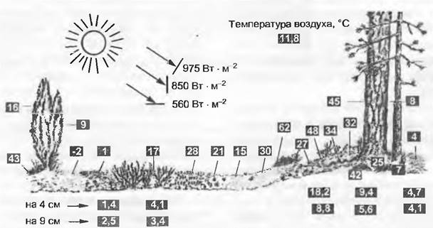
Due to relief, slope exposure, soil structure, and vegetation cover, the actual climate experienced by plants does not always match the data recorded by meteorological stations (Fig. 12.8). This microclimate can differ so drastically from the macroclimate that, at the level of an individual plant, differences between climatic zones periodically disappear. This effect is particularly pronounced in mountains, where low, dense plant communities strongly inhibit heat exchange with freely circulating atmospheric air, so that tropical temperatures can develop On the surface of the plant canopy during the day due to radiant heat. The lower and denser the vegetation stand, the more pronounced this climatic divergence becomes (it is stronger in meadows than in forests). Heat radiation on clear nights lowers the surface temperature of the vegetation below air temperature, which can result in unforeseen frost damage. Crucially, the vegetation cover acts as a climate modifier in its own right, altering all climatic components.

Fig. 12.8. Microclimate in the terrestrial living space. Spring situation at a forest edge in the Netherlands (noon after a clear night, March 3, 1976). An example of strong spatial diversity in the plant-level microclimate compared to air temperature (macroclimate). Solar radiation intensity varies depending on the angle of incidence on the irradiated surface

As an example of the complex combined effects of relief, microclimate, and secondary consequences, let us examine a dwarf shrub heath in the Central Alps (Fig. 12.9).

Fig. 12.9. Combined effects of relief, microclimate, and other modified biological factors, illustrated by a profile across an alpine dwarf shrub heath in the Central Alps (see also Fig. 12.13). Responses to differing living conditions in microhabitats under the same macroclimate lead to a characteristic vegetation zonation: A — meadow in a hollow bottom with Soldanella and mosses; B — stands of alpine rhododendron (Rhododendron ferrugineum); C — rhododendron stands with Vaccinium myrtillus; D — dwarf shrub heath dominated by Vaccinium uliginosum; E — Loiseleuria heath (Loiseleuria procumbens); F — lichen heath with bare patches caused by wind erosion; G — open vegetation with rosette and cushion plants and Juncus trifidus; H — dwarf shrub heath with Arctostaphylos uva-ursi and Vaccinium vitis-idaea; I — overheating patch; J — dwarf juniper stands (Juniperus communis ssp. alpina) with Calluna vulgaris and Vaccinium vitis-idaea; K — rhododendron stands with juniper

Relief structure influences solar radiation as well as the wind-driven and highly uneven distribution of snow. In hollows with persistent snow cover, the soil is well-moistened, but the growing period is severely shortened, increasing the vulnerability of weakened plants to various chionophilous fungi. On wind-swept dome-shaped summits, snow cover is often entirely absent in winter, exposing plants to low temperatures and intense solar radiation (potentially leading to frost desiccation). On sunny slopes near the soil surface, summer temperatures are particularly high, which can cause bare patches in the vegetation cover. On windward sides, similar bare spaces are frequently caused by wind erosion.

The distribution of various plant species accurately reflects small-scale habitat conditions within the dwarf shrub heath. By comparing different species, they can be broadly used as ecological indicators (see 14.3.3) and, through calibration against empirically measured values, assigned indicator values for specific habitat factors. This allows semi-quantitative data for acting ecological factors to be obtained for plant communities and their biotopes without time-consuming measurements.

In aquatic ecosystems, temperature and available radiation also deviate significantly from meteorological station climate data (Fig. 12.10). In spring and summer, the upper water layers predominantly heat up. Due to its shallow depth, the warm water remains at the surface in summer (epilimnion), while the cold and denser hypolimnion lies beneath it (Fig. 12.10, B). Cooling in autumn and winter, combined with wind action, promotes layer mixing, which is of decisive importance for the oxygen and nutrient supply of the entire water Column.

Fig. 12.10. Climatic conditions in the aquatic habitat: A — solar radiation; B — vertical temperature distribution during the summer months in a temperate eutrophic lake (Mondsee, Salzkammergut)

12.5.2.3. Soil

Soil is formed through the combined action of soil-forming factors: parent material, living organisms, climate, and topography, which act over time on pedogenic processes. The most important soil-forming processes are weathering, relocation, Humus formation, mineralization, and aggregation. Depending on the topographic position, this creates the living pedosphere, which represents a part of the biosphere. The edaphon is the totality of living organisms intrinsic to the soil. The rhizosphere encompasses the entire space occupied by roots and represents the contact zone between the vegetation cover and the soil. Soils are open porous systems consisting of solid, liquid, and gas phases, in which matter and energy are exchanged with the lithosphere, atmosphere, hydrosphere, and biosphere. Of great importance, especially for soil fertility, is the formation of clay minerals and humus. Humus is the organic component of the soil, generated by the edaphon through the decomposition and Processing of plant litter and its mixing with mineral soil constituents (Fig. 12.11).

Fig. 12.11. Leaf litter decomposition and humus formation (mull) in a beech forest on a brown forest soil: A — leaf litter; B — Skeleton feeding (springtails, etc.), exposing the epidermis (onset of bacterial and fungal colonization); C — transition to hole feeding; D — hole feeding and destruction of skeletal Veins (woodlice, centipedes, etc.), animal droppings; E — peak of microbial decomposition (bacteria, fungi), further consumption by saprophages (moss mites, etc.); F — ingestion of the decomposed mass, mixing it with minerals, and formation of a clay-humus complex aided by detritivores (earthworms, etc.); G — state after repeated gut passage (accelerated by bacterial decomposition!) and formation of a granular structure — mull humus (A – E — nearly 1 :3, F – G — approximately 150x)

In terms of mass and metabolism in the moderately humid zone, the most important soil organisms are earthworms and bacteria. Earthworms with a biomass of 20 — 80 g • m^-2 can process 10 — 40 t of fine earth per hectare per year. In subtropics and the tropics with a dry season, the dominant animal decomposers are termites (in Tanzania, for example, up to 200 termite mounds per 1 km² have been counted); they play a decisive role in mixing and heaping the soil (upon colony collapse). In steppe regions, constant soil mixing is ensured by various burrowing rodents (voles, ground squirrels, etc.).

Depending on base saturation, the accumulation of organic matter in the soil leads to a decrease in pH values, in extreme cases down to extreme values of about 3. All factors that retard the decomposition of plant material, such as poorly decomposable conifer litter, unfavorable climatic conditions, or base-poor parent rocks, promote the formation of mor humus and consequently soil acidification. This is closely linked to the mobilization and availability of mineral nutrients. Most plants, aided by mycorrhiza-forming fungi, are able to better utilize soil nutrient reserves and thereby increase biomass production.

Interactions between soil and vegetation are diverse and highly complex, preventing simple conclusions regarding cause-and-effect relationships. The determining factors for The structure of these interactions are the underlying parent rock and climate. Plants not only settle on specific soils but also influence soil formation. This process frequently leads to species turnover. The quality and quantity of litter (e.g., needles or leaves) are crucial for the dynamics of the topsoil layer.

Base availability, which can vary widely even within a single pH step within a buffer system due to soil acid buffering, is ecologically more important than the instantaneous pH value. The most important buffer systems correspond to the following pH ranges: carbonate — 8.6 — 6.2; cation exchange — 5 — 4.2; aluminum — less than 4.2; iron — less than 3.8; silicate — across the entire amplitude. Calcium content is particularly important. In addition to its significant buffering effect, it influences physical soil properties, such as structure (crumb structure), and thus the water, air, and thermal regimes.

Topsoil pH values typically fall within the following approximate ranges: 2.6 — 4.5 in strongly acidic raised bog soils and dwarf shrub heaths; 3.5 — 4.5 in acidic forest soils; 4.5 — 6.0 in rich, moderately to weakly acidic mixed deciduous forest soils and arable soils; 5.0 — 6.5 in fen soils; 6.0 — 7.5 in beech forests on carbonate rocks; 6.5 — 8.0 in floodplain forests; 7.0 — 8.5 in more or less alkaline steppe soils on limestone, up to 10 and more under arid halophytic vegetation (strongly alkaline soda soils are classified as solonetz).

Soil overacidification is caused not only by the formation of humic acids, but also by the release of acids by roots and microorganisms, the dissociation of carbonic acid, and base leaching. Because Plant Growth and soil organism activity are subject to seasonal fluctuations in precipitation and temperature, pH values follow a typical seasonal rhythm. Soil alkalinization is primarily driven by the accumulation of salts of strong bases and weak acids (e.g., Na₂CO₃, CaCO₃).

In forests, the majority of organic litter accumulates on the surface (litter layer). This directional input of litter leads to a very pronounced vertical Differentiation of the soil profile (Fig. 12.12). Under herbaceous vegetation and in typical steppe soils, organic litter is primarily supplied by the death of fine roots, which, along with The activity of burrowing animals and reduced infiltration due to dryness, explains the significantly lower vertical differentiation of humus content. The average residence time of carbon in the soil for certain components is measured in millennia; therefore, humus-rich soils are of considerable age, making their destruction over certain time periods final and irreversible.

Fig. 12.12. Soil development in the Atlantic climatic region of Europe. Soil stratification is clearly illustrated by its profile, which changes over time. Soils "mature" but can also degrade. The graph shows The sequence of pedogenic stages

The Classification of soil substrates is based on: 1) the parent material (e.g., limestone, silicates); 2) texture, the so-called grain size class subdivision; 3) humus content. The grain size classes adopted in Germany are listed in Table 12.1.

Table 12.1. Soil grain size classes adopted in Germany

* Values in parentheses are given according to international classes.

From an ecological perspective, aside from soil particle size, its structure is particularly important, which is determined simultaneously by pore volume and pore size classes, which are crucial for water retention (Table 12.2). Sandy soils have large pores, are well-aerated, drain quickly, and therefore have a low water-holding capacity (light, warm soils); loamy and clayey soils, by contrast, are heavy and cold. Compounds of colloidal clay minerals and humic substances (highly complex giant molecules comprising numerous aromatic rings with partially bound nitrogen and aliphatic side chains) form clay-humus complexes, onto the negatively charged surfaces of which exchangeable cations are bound. In undisturbed soils, root hairs, mycorrhizae, and microorganisms are so closely associated with these aggregates that nutrient leaching is extremely hindered. Due to the chemical binding of nitrogen in partially extremely inert humic substances, a large amount of nitrogen exists in a form unavailable to plants (C/N ratio in humus 10/20, in green leaves 30/50, see 13.6.1); consequently, data on the total nitrogen pool in soils provide no indication of plant nutrient supply. The maximum "loading" of soils with plant-available mineral nutrients is largely determined by the clay and humus content. According to a recently developed biogeochemical model, global productivity is ultimately limited by the clay content of soils. This raises the question: how much carbon can be globally bound in the biosphere?

Table 12.2. Pore size classes

Soil classification relies heavily on soil profile structure, i.e., horizon formation, which is typically designated by uppercase letters (see box 12.1). A distinction is made between organogenic and mineral horizons.

Principal organogenic horizons:

L — litter, largely undecomposed plant residues;

F — Fermentation or moder horizon (tissue structure is discernible);

H — humus horizon, organic residues without tissue structure.

Main mineral soil horizons:

A — topsoil horizon (strongly humified);

E — eluviation horizon (eluvial horizon);

B — illuvial mineral horizon (characterized by mineral neoformations and enrichment);

G — horizon influenced by groundwater;

S — horizon influenced by stagnant water;

C — parent material from which the soil has formed.

The naming of soil types relies on striking features such as color (brown earths, chernozem) or sequences of easily distinguishable horizons. A shift in soil types occurs when soil-forming factors change. If the soil-forming factors remain constant under a moderately humid climate, weakly structured primitive soils (A — C) later develop into illuvial soils (brown earths of the A — B — C type) or soil types formed under The Influence of redeposition processes (podzols A — E — B — C). In recently formed A — C type soils (e.g., rendzinas on limestone or rankers on silicates), the A horizon lies directly on the parent rock. Soil-forming factors can vary greatly over small distances, leading to a soil mosaic (Fig. 12.13). The A horizon is considered the donor and the B horizon the recipient for substances mobilized during soil development.

Fig. 12.13. Formation of a vegetation mosaic due to soil properties varying according to climate and topography. The example, as in Fig. 12.9, is taken from the alpine zone, where this soil Variability is manifested over particularly small areas.

The typical sequence of horizons in moderately cold coniferous forests as well as under tundra vegetation is as follows.

Humus occurs in the form of mor (raw humus), which lies on the mineral soil horizons and in which L, F, and H horizons of varying thickness can be distinguished. In the A horizon, above which Various Forms of raw humus lie, mixing of humic substances and mineral soil components takes place. In cold and moist regions, the A horizon is followed by a more or less bleached, humus-poor, or entirely humus-free eluviation horizon (E), which is characteristic of podzols. In this horizon, clay minerals are weathered to the greatest extent, and their weathering products are redeposited, such as Fe and Al containing humus sols. In extreme cases, the E horizon consists solely of quartz sand. In podzolic soils, the B horizon is therefore not only a weathering horizon but also exhibits clear signs of enrichment with substances, particularly iron-humus colloids. Under certain conditions, this horizon can become so impregnated with these substances (ortstein) that it becomes difficult for roots to penetrate. The transition from the B to the C horizon is mostly gradual.

This sequence of horizons is not yet expressed in young, primitive soils. Accordingly, in A—C type soils, the E and B horizons are absent and only begin to develop during soil formation under appropriate pedogenic conditions.

Under temperate conditions, roughly similar to those of deciduous forests, humus frequently occurs in a form known as moder, which is characterized by thin L, F, and H horizons. Under very favorable decomposition conditions, a form of humus called mull arises, in which the F and H horizons are completely absent. Mull is not a form of moder, since the mineral A horizon lies directly beneath the litter layer, with humic substances and mineral fine earth mixed together. Under such conditions, podzols do not form; instead, soils of the brown earth series, lacking sesquioxides and organometallic compounds, predominate.

In areas with high precipitation and in soils with impeded water percolation, waterlogged soils known as pseudogleys are formed, whi

ch, unlike gleys, are permanently saturated with groundwater.

In dry, warm continental climates of (forest) steppes and prairies, black soils (chernozems) predominantly form. These are very nutrient-rich, fertile soils of the A — C type with a thick, black-colored humus horizon that passes directly into the mineral substrate (often loess). To the depth of atmospheric precipitation penetration, lime is leached from these soils and redeposited in deeper horizons. In arid semi-desert and desert regions, the proportion of humus becomes increasingly smaller. Here, for example, chestnut-colored or gray soils (kastanozems, aridisols) are formed. In depressions of such areas, where scarce moisture can accumulate and infiltrate, high evaporation leads to the upward transport of soluble salts (e.g., Na₂CO₃, Na₂SO₄, NaCl, MgSO₄, etc.), which accumulate and form efflorescences on the soil surface. In such mostly strongly alkaline soils (solonchaks), the pH can reach 10. In the humid tropics, litter decomposes very rapidly and nutrient-poor lateritic soils are formed. Alkaline and alkaline-earth elements, as well as silicic acids, are leached from deeply weathered mineral soils, whereas iron and aluminum oxides, along with kaolinite, accumulate. These soils contain scarcely any large quantities of weatherable silicates (Box 12.1).

Box 12.1. Soil Classification

Due to the large number of different soil types, There is a need to group them into soil classes. Such classification facilitates communication among specialists and allows soil mapping based on similar features. To date, there is no universally recognized international system of soil classification. Currently, classification is carried out using three different methods, based either on soil-forming factors, soil-forming processes, or the Properties of the soils themselves. Classification based on soil-forming factors leads to the division of soils according to climatic and vegetation zones (zonal soils) or according to parent material type and topography (azonal soils). Typical zonal soils include boreal podzols, temperate brown earths, and tropical lateritic soils. Typical azonal soils include alluvial soils, waterlogged soils, or primitive soils.

Classification based on soil properties relies on precisely definable features of diagnostic horizons. This system was developed in the USA in the 1960s ("Soil Taxonomy") and is currently one of the most widely used classification methods, although it requires a significant amount of field and laboratory data. In most European countries, by contrast, soils are classified from a morphogenetic perspective, simultaneously taking into account soil-forming processes and habitat factors. This system is best suited for the pedogenetic interpretation of individual soils and has been somewhat modified in various countries to suit their specific conditions and needs.

A very widely used classification system is the FAO-UNESCO system, developed for the purpose of mapping the world's soil cover. In this system, classification is carried out based on diagnostic soil features as well as soil-forming processes and habitat factors.

Due to widely differing classification approaches, a strictly logical comparison of classification units across different systems is impossible and not always meaningful. Nevertheless, an attempt can be made to show how the most common soil types are represented in the three classification systems.

The US Soil Taxonomy recognizes 10 orders at the highest categorical level; the soil names are derived primarily from Greek and Latin roots (Table A).

Table A. US Soil Taxonomy

Table B. FAO Soil Classification

The FAO soil classification comprises 28 major soil groups (Table B), listing those of particular importance to Central Europe.

Table C presents a fragment of the classification system used in Germany, serving as an example of systems adopted in most European countries.

Table C. German Soil Classification System (fragment)