BOTANY VOLUME 4 - ECOLOGY - 2007

13. PLANTS IN THEIR HABITAT

13.7. Growth and Carbon Balance

The success of a plant species in colonizing its habitat ultimately depends on its ability to establish and maintain a viable population. This requires four conditions:

✵ the capacity for growth and biomass production under given resource availability;

✵ The ability to withstand typical environmental stress factors;

✵ the resilience to disturbances caused by herbivores, pathogens, or mechanical factors;

✵ successful reproduction.

Plant growth dynamics determine the chances for regeneration following stress or disturbance, competitive success for resources against other species, and The production of sexual offspring or clonal propagules. Therefore, understanding the processes that directly influence growth plays a priority role in plant ecology. Following An Overview of growth ecology, subsequent sections address biomass production and ecosystem carbon balance. These are underpinned by the PHYSIOLOGICAL AND BIOCHEMICAL principles of Photosynthesis and Respiration (see 6.5, 6.10).

13.7.1. Ecology of Photosynthesis and Respiration

Photosynthetic CO₂ fixation and respiratory CO₂ release form The basis of the global carbon cycle (see 13.7.6). Both processes, In addition to internal factors, are strongly dependent on environmental conditions. Because photosynthesis and respiration—including decomposition-related respiration following plant mortality—involve comparable quantities of carbon fluxes, they are attributed equal importance in the carbon balance. Nevertheless, a great deal is known about photosynthesis, whereas respiration remains comparatively understudied. This is likely because photosynthesis takes place in well-defined and readily accessible Organs (typically green leaves), whereas respiration involves all plant organs, including subterranean ones, and varies significantly depending on the organ type.

Since photosynthesis is driven by light, specifically the photosynthetic photon flux density (PFD), it is customary to express its rates relative to the projected area of assimilatory organs (leaf area). Respiration rate R is independent of directional vectors, and thus it is preferable to derive it from tissue quantification metrics (most commonly dry mass). For leaf respiration rates, particularly at the ecosystem scale, surface area-based ratios are also utilized. The choice of reference metric has a decisive impact on the results and the resulting Conclusions. CO₂ fixation is simultaneously counteracted by CO₂ losses via Photorespiration and mitochondrial respiration in leaf Tissues. Typically, only the net outcome—the net photosynthetic rate A (assimilation)—is accessible to observation. Because mitochondrial respiration is partially inhibited in the light, and photorespiration assumes crucial Functions in maintaining the photosynthetic machinery under fluctuating light regimes (see 6.5.6), it is neither ecologically meaningful nor recommended to add dark-measured respiration rates or even photorespiratory "losses" to net photosynthesis to calculate gross photosynthesis.

A major challenge in characterizing the dependencies of A and R on external factors is that these relationships vary greatly over time and, in turn, depend on other variables. Thus, rather than having a fixed "reaction norm" for a given species, an entire array of such functions and their rapid shifts in response to environmental conditions "regulate" the functional dependence. Since the General Principles were outlined in sections 6.5 and 6.10, this section will focus exclusively on ecologically significant interactions (Fig. 13.30; for CO₂, see Fig. 13.45).

Class="center">Fig. 13.30. Interactive dependence of leaf photosynthesis on light, Temperature, and CO₂ concentration in C₃ plants (schematic): A — change in the response to photon flux density (PFD) when 600 ppm CO₂ is supplied instead of 360 ppm; LKP is the light compensation point at 360 ppm CO₂; B — change in the response to temperature under a gradual decrease in PFD (down to 5% of PFD_sat) at a normal CO₂ concentration. The CO₂ response curve is identical in shape to the PFD response curve (cf. Fig. 13.45). For further details, see text

The functions in Figs. 13.30 and 13.45 are characterized by boundary values and specific curve segments. The intercepts on the abscissa are referred to, in the case of the PFD and CO₂ dependencies, as the light and CO₂ compensation points (both given for sun leaves of C₃ plants and fortuitously matching in value at 20 °C, around 20–30 µmol photons • m^-2 • s^-1, or ppm CO₂). The linear initial slope of both saturation functions is designated as the quantum use efficiency (QUE) and CO₂ uptake efficiency (CUE). The linear rise of the PFD curve represents rate limitation by

the light-dependent reactions of photosynthesis (regeneration of CO₂ acceptors, RuBP), whereas the plateau of the curve (saturation) represents limitation by the dark reactions (CO₂ fixation, carboxylation). The opposite holds true for the CO₂ curve: the initial rise reflects limitation by the dark reaction, while the plateau reflects limitation by the provision of reduction equivalents (light reaction). CO₂ concentration and PFD interact in such a way that with increasing CO₂ concentration, the light compensation point shifts to the left (towards zero), and PFD saturation for A is reached at higher PFD values. Ecologically, this means that light is utilized more efficiently at elevated atmospheric CO₂ concentrations, especially in the shade (see 13.7.6). Both the light compensation point and light saturation are highly adaptive. Shade plants compensate at PFD <10 (down to 3) µmol photons • m^-2 • s^-1 and saturate at 100–150 µmol photons • m^-2 • s^-1 (approximately 5–8% of full midday sunlight). Most sun plants achieve 90% PFD saturation at 400–600 µmol photons • m^-2 • s^-1, whereas leaves with exceptional thickness and structural robustness reach saturation only at PFD >1000 µmol photons • m^-2 • s^-1 (for C₄ and CAM plants, see 6.5). Although the dependence of A on CO₂ also exhibits acclimation behavior upon prolonged exposure to elevated CO₂ concentrations, it does not remain constant (see Fig. 13.45).

The temperature dependence of A is a complex function resulting from promoting effects (Rubisco carboxylase activity) and inhibitory effects (Rubisco oxygenase activity + mitochondrial respiration), which together generate a bell-shaped normal distribution curve. The lower and upper boundary values (A = 0) and the optimum (A_max) are characteristic of specific climates. In temperate, boreal, and arctic-alpine regions, during full leaf activity, the temperature thresholds of frost hardiness coincide with the temperature thresholds for A (–2 to –8 °C, often around –5 °C in mountain regions). This means that A ceases when leaves are irreparably damaged

by frost to the point of death. The upper temperature threshold lies between 40 °C (cold-adapted plants) and 45 °C (heat-adapted plants), meaning it is also separated from lethal overheating by only a few degrees (see 13.3.2). The optimum ranges between 15 °C (extreme cold-adapted plants) and nearly 30 °C (heat-adapted plants). Even lower optima are observed in cryptogamic plants of cold biomes.

The optimum can shift by 5 K (or more) within a short period of time (a few days) through acclimation. The actual (micro)climate is the decisive factor for adaptation. Since cushion plant communities in the mountains receive relatively high temperatures in the sun, it is hardly surprising that their photosynthetic temperature optimum is very similar to that of lowland plants (20–25 °C). In temperate and cold regions, the temperature optimum for A is very broad (90% of A occurs within a range of >10 K). In tropical plants, A drops to 0 already at the cold boundary (3–7 °C), and the optimum is comparatively narrow.

The interrelationship between light and temperature is of great ecological significance. The PFD and T dependencies discussed above apply to optimal temperature and light saturation, respectively. While such response functions can be measured in the laboratory, they are manifested to a very limited extent in nature. This is because during the growing period (with few exceptions), high PFD coincides with warmth, whereas strongly limited light coincides with coolness. The photosynthetic apparatus of plants is well-tuned to this. The interactive effect of PFD and T is such that at low PFD, the temperature optimum for A is also reached at much lower temperatures (e.g., 12 °C instead of 22 °C). Under low light conditions, plants achieve the highest possible photosynthetic rate for these limiting conditions at a relatively low temperature. Therefore, photosynthesis is almost never limited by temperature, but frequently by light. Leaf photosynthesis measured under light saturation, optimal temperature, and "normal" CO₂ concentration is now referred to as the maximum photosynthetic rate A_max. The term photosynthetic capacity A_cap, previously used for this, is now reserved for the maximum possible photosynthesis under CO₂ saturation.

Capturing respiration in a realistic manner and establishing convenient standard parameters that do not yield discrepancies are among the toughest challenges in functional ecology. Three types of mitochondrial respiration are distinguished: maintenance respiration (referred to hereafter simply as maintenance respiration), so-called growth respiration associated with The formation of new tissues, and nutrient uptake respiration in roots. The intensity of maintenance respiration R strongly depends on tissue activity, but it is modulated by The ratio of dry weight to carbon content in the tissue—i.e., its spatial density (the denser the tissue, the lower the calculated respiration intensity per protoplast), which in turn affects the nitrogen concentration relative to dry weight (see 13.6.3). Flowers, fine roots, and leaves (in the dark) exhibit high R values per gram of dry weight, stems and thick roots lower values, and woody structures or storage organs very low values. When based on nitrogen content (as a proxy for protein), these differences often vanish or become very small. As a general rule, an active plant consumes roughly half of its daily CO₂ assimilation in respiration, and "soft" tissues account for the largest share of these losses relative to invested carbon (dry weight).

Comparing the respiratory activity of different organs, plant species, or even individuals of the same species from different habitats invariably involves accounting for Environmental Effects on the calculated parameters. In other words, the environment or developmental stage influences Cell-specific respiration so strongly that actual values frequently deviate from theoretical parameters (such as tissue bulk density). Finally, maintenance respiration is extremely sensitive to

all conceivable influences, including internal plant developmental changes, assimilatory activity, prior stress exposure, and especially destructive interventions such as ROOT excavation. Since roots account for the majority of "total respiration costs" in many plants, a major difficulty lies in the fact that determining the respiration of roots in an intact rhizosphere is only possible indirectly (e.g., using ¹³C isotopes) and at a very high methodological cost.

Temperature is the most critical climatic variable for the respiration of active plants (see 6.10.3.6). In general, R doubles with rising temperature (like the norm for most enzymatic processes) when the temperature in the intermediate range (e.g., 10–20 °C) increases by 10 K (Q₁₀ = 2). From an ecological perspective, the Effect of temperature on respiration cannot be adequately described by this rule alone, which represents merely a special case. Scarcely any other life process reacts so dynamically to changing conditions as mitochondrial respiration. The founder of modern field-oriented ecophysiology in Germany, O. Stocker, was likely the first to be astonished to find that adjustments of respiration to prevailing temperatures are so pronounced that they can compensate for even the widest temperature amplitudes.

Stocker compared the summer (shade) respiration of willow (Salix) in its natural habitat in Greenland with that of tree branches in the humid tropical rainforest of Indonesia, finding no differences between them. Similar observations were made by A. Pisek, who investigated the respiration of conifers in a valley and at the upper timberline in Tyrol. However, when the respiration of plants or tissues from warm and cold regions is measured immediately after sampling at identical temperatures (rather than the temperatures prevailing in their natural habitats), it becomes apparent that the respiration rate of cold-adapted plants is consistently and distinctly higher. In literature, this is often misinterpretated as "more intense respiration in cold regions." In reality, respiration in cold regions tends to be lower, primarily due to cold nights. The Conclusion that plants attempt to counteract unfavorable temperature conditions by increasing specific activity is supported by the observation that the number of Mitochondria increases as the habitat temperature decreases. Respiration should not be viewed merely as a burden on the carbon balance; rather, it is a vital metabolic process (a "requirement").

Acclimatization adjustment of respiration to new ambient temperatures (Fig. 13.31) proceeds relatively quickly (from one to several days), but is not always complete, as shown in this example. The graph clearly demonstrates that it is inappropriate to forecast actual process rates in a thermally dynamic environment (such as global climate change) based solely on known short-term temperature dependencies of metabolic processes. Such projections must account for the acclimatization capacity of plants.

Fig. 13.31. Temperature dependence of respiration before and after acclimatization. The bold arrow indicates the direction of acclimatization to a higher temperature new to the plant (20 °C instead of 10 °C), with each curve representing the short-term respiratory response to various temperatures (within the experimental duration of 1–2 h) in groups of plants of the same species adapted to either cold or warmth. In this example, warm acclimatization is either partial (a) or complete (b). In case b, this means that after acclimatization, the plant group placed in warmth respires at the new temperature with the same intensity as previously in its colder natural habitat. At identical temperatures, the 20 °C-acclimatized group respires at a lower intensity than the cold-acclimatized group, though this is ecologically insignificant. NA marks the theoretical respiration intensity at the new growth temperature if no acclimatization had taken place. Curve a represents the most frequent case

13.7.2. Growth Ecology

Ultimately, plant growth represents the balance between income and expenditure expressed in dry weight, i.e., the sum of assimilated carbon minus the sum of all respiration costs and other losses. The rate of net carbon fixation by the entire plant over a given period depends on factors such as:

✵ photosynthetic rate per unit of leaf area (integrated across all leaves);

✵ the ratio of total leaf area to total plant biomass (leaf area ratio, LAR);

✵ respiration of all organs (which varies greatly among different organs);

✵ carbon export (e.g., to symbionts);

✵ The activity of carbon deposition (structural growth or storage).

Each of these 5 factors is, in turn, dependent on numerous external and internal influences. It is impossible to predict carbon fixation or growth based on a single factor alone. This simple realization stands in contrast to the long-dominant view that growth is a direct consequence of leaf photosynthesis and is limited solely by its activity rate. This unfortunate tunnel Vision resulted in a wealth of knowledge regarding photosynthesis in nature, while very little—or almost nothing—was known about the other 4 growth determinants and their environmental dependence. Although all four additional factors can theoretically influence net C production quite effectively, 3 of them (excluding the last one) vary in a given plant species only within certain morphologically constrained limits. Conversely, C-deposition activity, regulated by other available resources (actual mass increment), is extremely variable and in most cases (except under light limitation) constitutes the direct driving force governing carbon assimilation by the plant. This becomes evident from the simple fact that photosynthesis proceeds unhindered as long as the produced assimilates find utilization somewhere within the plant itself, i.e., can be invested. Otherwise, "production" must cease immediately, as transport pathways quickly become "clogged" and METABOLISM/14.html">Chloroplasts consequently overflow with assimilates (end-product inhibition).

From an ecological standpoint, this is the central point for understanding plant growth.

High carbon deposition activity induces a high photosynthetic rate, whereas low activity decreases it. If accumulated carbon is removed from the plant—for instance, via growing potato tubers or apples—the photosynthetic rate in the leaves drops. If a plant is deprived of a portion of its leaves, the photosynthetic rate in the remaining leaves increases.

The activity of carbon deposition in a plant depends on the availability of soil resources (Water and nutrients), temperature, and the developmental stage of the plant itself, which in turn is determined by the two preceding factors and numerous others (e.g., photoperiod). Extensive literature confirms that carbon deposition activity responds to all environmental influences, with the exception of light, and is more sensitive than leaf photosynthesis. Growth processes (Cell Division, expansion, and differentiation) respond long before photosynthesis is significantly constrained by water scarcity, mineral nutrient deficiency, or low temperatures. Therefore, it is no exaggeration to state that in most cases—barring light limitation (and naturally situations following leaf loss)—growth, and thus the demand for assimilates, governs photosynthesis rather than the other way around.

It is remarkable how long this has been known and how little it has been applied in general biological paradigms. In 1864, E. Kraus published the results of a classic experiment in the journal *Flora*, which he conducted in Julius Sachs's laboratory in Würzburg. At that time, photosynthetic activity in leaves was still determined by observing gas bubble formation in water-submerged shoots. Sachs's co-workers were already aware that the rate of photosynthesis is occasionally decoupled from assimilate demand and export rates, leading to enhanced formation of assimilation starch, which could be demonstrated using iodine and potassium iodide. Kraus posed a highly modern question: which of the two processes is more severely affected by low temperatures—photosynthesis (gas bubble formation) or assimilate utilization (starch accumulation)? The answer was provided by ice cubes dropped into a water bath: in the cooled water bath, bubble formation barely decreased, whereas The amount of starch increased compared to the warm control water. Despite all valid modern objections to such an experiment from a contemporary perspective, the train of thought and observations brilliantly illustrate the dilemma: what limits carbon assimilation—its deposition or its supply source? Recent findings for plants from cool regions have united all this into a coherent picture: at 0 °C, leaf photosynthesis still achieves about a quarter of its maximum possible productivity and only ceases around -6 °C (see Fig. 13.30, B); conversely, growth—i.e., deposition activity—ceases at temperatures just above 0 °C and proceeds very slowly below 5 °C. Accordingly, uncommitted CARBOHYDRATES (starch, fructose) and, over longer periods, Lipids accumulate in the plants of cold biomes. A complete analogy exists during seasonal drought periods, as growth is likewise far more sensitive to moisture deficit than photosynthesis.

Respiration often responds to environmental factors (especially temperature) to a much greater degree than photosynthesis, partially dampening deposition activity (growth respiration), yet it is extremely difficult to quantify due to organ-specific variations. For instance, it is practically impossible under natural conditions to measure root respiration, which is typically the largest source of carbon loss. As soon as fine roots are excised from their microenvironment and separated from symbionts, their respiration pattern changes.

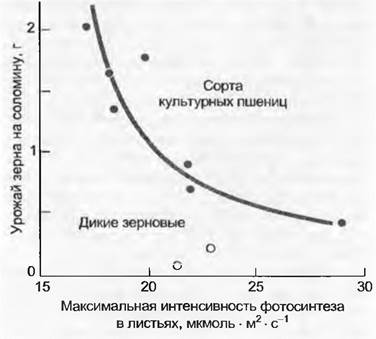
The Significance of carbon deposition—and consequently the pattern of assimilate investment—is a central issue not only in ecology but also in agricultural science. Aside from agronomic management practices, increasing grain crop yields essentially boils down to directing assimilation flows toward the desired end product rather than achieving higher leaf activity (Fig. 13.32). Prominent researchers have repeatedly demonstrated that increased grain yield is not correlated with enhanced leaf photosynthetic rates.

Fig. 13.32. Maximum photosynthetic rate $A_{max}$ in leaves and grain yield. A classic example from agricultural practice demonstrating that photosynthetic productivity per unit of leaf area does not determine yield. In this example, the relationships between yield and photosynthesis are even negative for various wheat varieties. Leaves of two wild-growing species of the genus Aegilops exhibit $A_{max}$ values no lower than those of modern high-yielding varieties (each measurement point represents the mean of numerous individuals of a given variety/species). Yield-determining factors include stem and spike Morphology, dry matter partitioning (harvest index), leaf adaptation to low light (enabling them to produce even in the lower canopy layers), leaf lifespan, and the intrinsic developmental rhythm (delayed senescence) of the entire plant

A short-term net profit calculation alone can contribute very little to an ecological understanding of the growth process. This becomes even more challenging over longer observation periods when the question of the functional lifespan of all organs and tissues arises (amortization issues). The "profit" accrued by a leaf results from the balance between the lifetime production of photosynthetically fixed $CO_2$ and the construction costs of the leaf itself, minus the export of remobilized substances prior to its senescence. Disregarding cost considerations, yield is the product of work per unit time multiplied by its duration; both values are equally significant. Although radiation-to-protein ratios (nitrogen content) per unit leaf area can yield a relatively accurate prediction of photosynthetic rate (see Fig. 13.20), such measurements involve high effort and expense. In contrast, literature data regarding leaf lifespan remain extremely scarce, even though such information can be easily obtained without technical overhead.

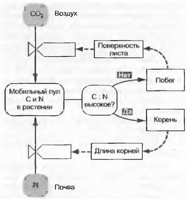
Growth is determined by where and in what form carbon assimilates are invested. The remobilization of photoassimilates into new leaves is expressed in compound percentages (daily percentages!). Investment in green stems may be neutral from a balance perspective, whereas costs for storage organs are lower, and those for fine roots are higher (primarily due to respiration costs). Such "decisions" are not "free"; they are governed by three driving forces: the bauplan, i.e., the inherited morphotype; the developmental type and concomitant shifts in primary investment sites throughout the lifespan; and external factors. Assimilation flows are regulated within boundaries dictated by Cytology/cytology/67.html">Development and Structure, as well as resource availability (Fig. 13.33; cf. 13.7.3): high light—few leaves; low light—many leaves; high nitrogen availability—large leaf mass and small root mass, etc.

Fig. 13.33. A simple model illustrating the linkage between carbon and nitrogen budgets in a plant. Based on the question of whether There is a limitation of carbon (absorbed but not yet structurally fixed into photoassimilates) or nitrogen (available nitrogen compounds), i.e., mobile "building blocks" regarding the C/N ratio, their investment is directed preferentially either toward the leaves or, conversely, toward the roots. Solid arrows symbolize mass fluxes, while dashed arrows indicate regulatory effects

In forbs, grasses, dwarf shrubs, and tree seedlings, some of these growth determinants can be determined quite simply using a balance and a drying oven. They are at least as important as $CO_2$ acquisition relative to leaf surface area. It remains puzzling why, given scarce research funding (even in research-oriented countries), expensive gas-exchange apparatuses are deployed first, when equally rigorous investigations of other growth parameters could be conducted using much simpler means.

Depending on the carbon investment in leaves, a plant can acquire more or less carbon, thereby regulating the photosynthetic "yield" of the entire plant without altering the specific efficiency of photosynthesis. Besides light, the most critical parameters determining growth are temperature, available water, and nutrients. These factors dictate how much photosynthesis the entire plant can "afford" or how many assimilates can actually be "invested." This concept of demand-driven assimilate mobilization contradicts the prevailing view that growth is determined solely by the available pool of assimilates and, consequently, by photosynthetic productivity. The latter holds true only when all other growth factors are non-limiting. This occurs exclusively under specific conditions, such as intensive agriculture or deep shade, where CO₂ fixation becomes the sole determining factor. Characteristically, many evergreen plants accumulate reserves during dry periods (referred to as stored growth), despite limited CO₂ assimilation, and generally do not experience "starvation" during this time. With the onset of rains, these reserves are mobilized to support The Development of new shoots.

Although C₄ plants generally exhibit higher photosynthetic productivity than C₃ plants, their agricultural yield under high soil moisture conditions is not always correspondingly greater. They gain a competitive advantage under low water availability, particularly during droughts. Thanks to compensatory root growth, water and nutrient deficits may be temporarily masked, but natural limits are ultimately imposed at the ecosystem level. As recent studies in CO₂-enriched air demonstrate, stimulating the rate of photosynthesis with elevated carbon dioxide levels yields only a marginal increase in growth, since such experiments do not overcome growth limitations imposed by other scarce resources.

13.7.3. Functional Growth Analysis

Functional growth analysis is based on several core parameters that primarily concern how assimilates are distributed among various plant organs and how they are deployed within them. The environment can influence these allocation processes such that assimilates are preferentially invested where they are in short supply: in roots under soil drought, in leaves under light deprivation, and so forth. This is reflected in the dry mass of organs relative to the total dry mass of the plant (Fig. 13.34). In English nomenclature, the following terms are used for this purpose:

✵ LMF — leaf mass fraction;

✵ SMF — stem mass fraction;

✵ RMF — root mass fraction.

Similarly, reproductive organs, storage organs, and others can be designated as biomass fractions. Accumulating evidence suggests that these biomass allocation models do not always conform to the "functional equilibrium" originally described by H. Brouwer, and that dry matter partitioning responds very dynamically to environmental factors. Typically, physiological and morphological corrections (such as The regulation of nitrogen status and leaf photosynthetic capacity, cuticle properties, and leaf dimensions) are incorporated into this established model.

Fig. 13.34. Biomass allocation and plant life strategies. Photosynthetic organs account for vastly different proportions of total biomass. Shown here is the leaf mass fraction (LMF), expressed as the ratio of leaf biomass fraction to total biomass (% dry mass, shaded plane) in adult plants of various morphotypes representing different life strategies.

At the leaf and root level, we are interested in the biomass "cost" required to establish a functional unit. Since The primary function of leaves is Light absorption, it is best described in terms of leaf surface area. For roots, it is the intensity of soil exploration, hence the length of fine roots per unit of biomass. It is the root surface area that comes into direct contact with the soil, although the quality (activity) of this surface changes as roots age. When evaluating root surface, one must neither underestimate The Role of highly active, absorbing fine roots nor overestimate the role of older, thicker roots that no longer absorb water and nutrients (acting primarily as transport channels). Therefore, regardless of thickness, root length is frequently used as a functional measure. The corresponding parameters are designated as:

✵ SLA (specific leaf area — square meters of leaf surface area per gram of dry weight, or for clarity — dm² • g^-1 or m^-2 • kg^-1);

✵ SRL (specific root length — meters of root length per gram of dry weight).

Instead of SLA, the reciprocal value, LMA (leaf mass per area), is often used. Combining organ mass fractions and their specific "costs" yields two important equations of functional growth analysis:

LAR = LMF • SLA

(leaf area ratio — total leaf surface area relative to the total biomass of the whole plant, m² • g^-1);

RLR = RMF SRL

(root length ratio — total root length relative to total plant mass, m • g-1).

Meanwhile, numerous studies confirm that LAR represents a critical determinant of growth (Fig. 13.35), with both LMF and SLA potentially acting as decisive variables for the LAR value.

Fig. 13.35. Growth regulation via assimilation and investment. Relative growth rate varies independently of the total CO₂ assimilation rate of all leaves combined (ULR — unit leaf rate), but correlates linearly with the leaf area ratio (LAR). The dependence on LAR is predominantly driven by the SLA component (leaf surface area per dry mass) rather than the leaf mass fraction relative to total biomass (LMF). Data compiled by H. Poorter and A. Van der Werf for 51 different herbaceous plant species under optimal growth conditions.

LAR is primarily a static variable. An Assessment of the specific carbon fixation productivity of the leaf surface is also required. This is designated as ULR (unit leaf rate) and is defined as the increase in total plant dry weight per 1 m² of leaf surface area per day (g • m^-2 • day^-1). From this, the relative growth rate RGR of a plant is derived:

RGR = ULR • LAR.

The relative change in total plant mass M with respect to initial mass per day is given by:

RGR = 1/М • dM/dt (g • g^-1 • day^-1, or % • day^-1).

ULR provides an integrated measure of leaf assimilation productivity relative to the resulting net plant growth, reflecting carbon assimilation much more realistically than short-term leaf photosynthesis measurements. The drawback of ULR is that it can only be determined destructively (via biomass gain over relatively short intervals, such as a week) and is therefore restricted to herbaceous or at least small plants. For trees, wood increment and litter production can be roughly correlated with LAI. Because growth is heavily influenced by a "compound interest" effect and the trajectory of growth curves over time is rarely linear, dividing annual plant growth by the length of the growing season and treating the result as RGR is incorrect. A measure used in agriculture for plant growth productivity over longer periods (several weeks or months)—which serves as a calculated synonym for ULR, known as net assimilation rate (NAR)—denotes biomass increment per unit of averaged leaf surface area over a single, typically longer observation period. However, relating this to a leaf surface area that fluctuates rapidly over such an extended timeframe remains problematic.

RGR varies by up to two orders of magnitude depending on the species. In trees, LMF and RMF are more or less conventional, since growth driven by the accumulation of massive, inactive heartwood is very minimal. When calculated relative to the active conducting wood, however, the LMF and RGR values for trees are nearly identical to those of perennial herbs. Due to the daily "interest payments" on leaf growth, RGR can very rapidly reach extremely high values; a 20% daily biomass increase is not uncommon in young herbaceous plants. Meanwhile, numerous analyses confirm that fast- and slow-growing plants differ primarily in their biomass allocation relative to leaf surface area and total root length. In contrast to slow-growing plants, fast-growing species exhibit higher values of SLA (see Table 13.1 in Section 13.6.2) and SRL. Typical values for these parameters are listed in Table 13.2.

Table 13.2. Parameters* of functional growth analysis

* Rough baseline figures for well-developed yet non-senescent individuals in nature; numerical values may deviate significantly in seedlings, juveniles, and senescent specimens. LMF, SMF, and RMF are expressed in g • g^-1, LAR in m² • kg^-1, and RGR in g • g^-1 • day^-1 (all relative to total plant dry weight); SLA is expressed in m² • kg^-1, and SPL in m • g^-1 based on dry tissue weight (of leaves or roots).

Fig. 13.36. Model of the functional relationship between C and N allocation and assimilation and leaf lifespan. Only internal regulators of Plant Growth and nutrient availability are considered, omitting external factors such as climate, soil moisture, developmental processes, and biotic interactions (A = photosynthetic production, LAR = leaf area ratio, SLA = specific leaf area)

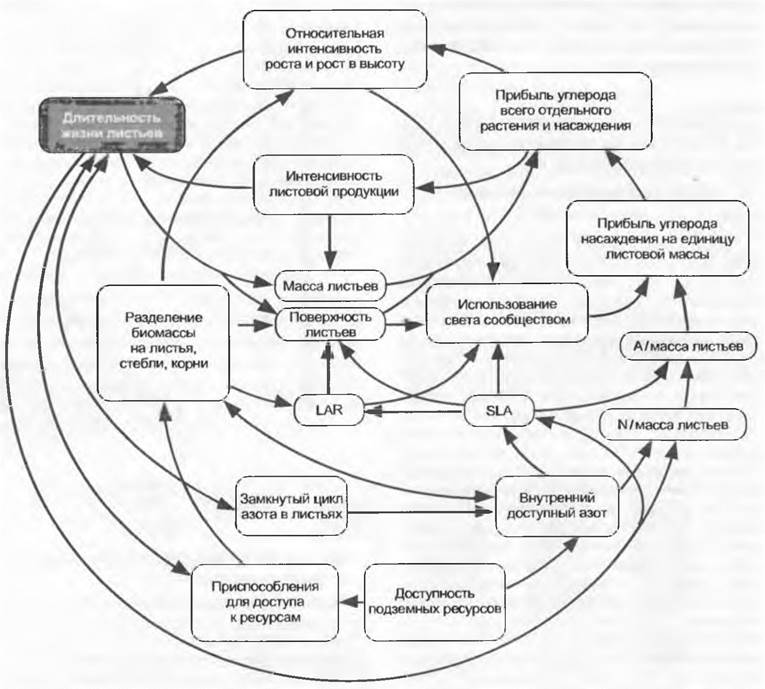
Fig. 13.36 schematically illustrates the coordination among the key determinants of functional growth analysis, showing (via curved arrows) how an individual leaf contributes to carbon gain within a monoculture. This functional model would become even more complex if one attempted to incorporate the multifaceted (and largely unknown) interactions with symbionts, herbivores, pathogens, and decomposers, or to understand the mechanisms of developmental processes (such as flowering) in light of these factors. This complexity increases further when above- and below-ground interactions among different plant species and age groups are factored in at the community level. Consequently, plant community growth cannot be predicted (modeled) mechanistically based solely on the functions of a single leaf, as data for countless parameters are missing. Such parameters are largely elusive because they represent variables dependent on other variables. The frequently used analogy of a mechanical system of gears and drive belts is misleading, because in the real world of plants, "the wheels vary in size, shape, and number of Teeth while the engine is running, the drive belts stretch under tension," and furthermore, the operational program (development) changes rapidly. Every prediction of plant growth is therefore statistical in nature, resting on trends and probabilities derived just as much from historical statistical observations. This has long been recognized in crop science. The complexity demonstrated here explains why one cannot expect genetic interventions in a specific isolated process (such as those occurring on chloroplast membranes) to yield predictable growth outcomes under natural conditions.

13.7.4. Stable isotope ¹³C in ecology

New methodologies often serve as the starting point for paradigm shifts in science. No other scientific breakthrough has had a greater impact on process-oriented ecological research since the mid-1970s than the discovery that naturally occurring stable isotopes of vital chemical elements such as hydrogen, nitrogen, oxygen (see 13.5.4, 13.6.4), and carbon are either enriched or depleted in plants relative to their surrounding environment. These isotopic signatures propagate through food chains, benefiting animal ecology just as much as plant ecology. The most significant among them is the ¹³C isotope. It accounts for 1.1% of all carbon in rocks, the atmosphere, and living organisms, with ¹²C making up the remaining 98.9%. The radioactive isotope ¹⁴C, which is continuously formed in trace amounts in the upper atmosphere—whose relatively rapid decay is used for dating organic material and which also serves as a tracer in analytical studies—is not discussed here.

Compounds containing a heavy isotope tend to diffuse slightly more slowly than identical compounds bearing the lighter variant of the same element, and in many cases, reaction rates are reduced. This phenomenon is known as physical and biochemical stable isotope fractionation. In the case of carbon, this primarily involves The transport of ¹³CO₂. Here, fractionation occurs such that CO₂ containing the heavier ¹³C isotope is discriminated against in plant tissues relative to CO₂ containing the lighter ¹²C isotope; in other words, ¹³C occurs in lower concentrations compared to its Abundance in the atmosphere (Box 13.1).

Box 13.1. Tracking carbon and water dynamics using δ¹³C

The primary analytical instrument for measuring isotopic ratios is the mass spectrometer, which is increasingly becoming standard equipment in biological research. Sample sizes required are within the milligram range. The technique must be capable of detecting a 0.1‰ difference in the ¹³C/¹²C isotopic ratio. Rather than absolute concentrations, researchers typically examine the relative deviation of the ¹³C/¹²C ratio in a sample from a standard ratio. The internationally agreed-upon reference material used to calibrate all ¹³C/¹²C measurements is Pee Dee Belemnite (PDB) limestone, whose δ¹³C content is defined as 0‰. The δ¹³C value of any other substance is calculated relative to this standard using the following equation:

Atmospheric CO₂, from which plants derive their δ¹³C, currently has a value that differs by -8‰ from the belemnite standard. This value is becoming increasingly negative due to the combustion of fossil fuels. In the 19th century, it was less than -7‰ (reconstructed from air trapped in melted polar ice). Instead of expressing isotopic ratios relative to belemnite limestone—which yields negative δ¹³C values—an alternative measure, discrimination against ¹³C (denoted as Δ), is evaluated relative to the atmosphere:

The magnitude of ¹³CO₂ discrimination during photosynthesis provides insights into critical steps of CO₂ uptake (stomatal diffusion and carboxylation). Because assimilates incorporate their isotopic "signatures" and are long-preserved in structural plant tissues, δ¹³C values serve as a mirror of assimilation conditions, both during contemporary plant growth and over thousands or even millions of years. The relationship between gas exchange and ¹³C discrimination was formulated by G. Farquhar and has been repeatedly confirmed by experiment:

corresponding to δ¹³C_sample = δ¹³C_air + a + (b - a) p_i/p_a (where a = 4.4‰, fractionation via diffusion; b = 28‰, fractionation via carboxylation; p_i and p_a represent internal and external partial pressures of CO₂, respectively).

Since p_a is known, p_i can be calculated via Δ, yielding information on stomatal limitation of gas exchange during assimilate formation from minute tissue samples. A low p_i indicates restricted stomatal aperture and, consequently, water stress.

Physical discrimination—essentially diffusion through stomatal pores—is weak and results in very little ¹³C depletion beneath the epidermis (-4.4‰).

This ¹³C-depleted CO₂ is subsequently bound by the enzyme RuBP carboxylase/oxygenase (Rubisco), a process during which ¹³C discrimination is substantially more intense, reaching up to 28‰. If initial fixation is carried out by PEP carboxylase (in C₄ and CAM plants), this additional fractionation does not occur because the enzyme does not alter the integrity of CO₂. In such cases, overall discrimination is restricted to stomatal limitation (4.4‰). Some minor ambiguities arise in C₃ plants because respired CO₂ derived from substrate already depleted in ¹³C may be refixed, which can play a notable role when stomatal aperture is small. Thus, total discrimination is always pronounced (strongly negative δ¹³C values) when Rubisco-mediated discrimination dominates (C₃ plants with wide-open Stomata), and minimal (less negative δ¹³C values) when stomata are heavily constricted, hindering CO₂ uptake, or in C₄ and CAM plants. Given an initial atmospheric value of -8‰, theoretical δ¹³C values can never be less negative than -12‰ (-8 + -4; C₄ plants) nor more negative than -36‰ (-8 + -28). In reality, well-watered C₃ plants average around -28.5‰ (frequently -25 to -32‰), whereas C₄ plants range between -12 and -14‰. In CAM plants, values depend on whether metabolism operates entirely via the CAM pathway or whether assimilation occurs via the C₃ pathway during humid weather (mostly falling between -13 and -20‰). The ecological utility of this information is self-evident.

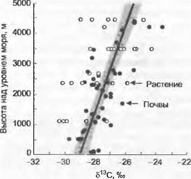
Using δ¹³C values, even minute samples of dead plant material (as well as herbarium specimens and fossilized plants) can be used to distinguish between C₃ and C₄ plants and, most interestingly, to determine whether C₃ structures developed under water deficit (less negative δ¹³C) or ample water supply (strongly negative δ¹³C). Fat, bone, or teeth samples from animals can reveal whether and when they grazed on C₄ vegetation. Soil humus samples can indicate whether they originated from C₃ or C₄ plant residues, providing evidence of historical vegetation shifts. This method has successfully demonstrated, for instance, that fossil Mollusks from the modern Negev Desert fed on well-watered C₃ plants thousands of years ago (indicating a humid climate), that C₄ plants have consistently predominated during geological epochs with low atmospheric CO₂ levels, and that carboxylation limitation is relatively minor in the leaves of high-altitude plants worldwide compared to related lowland species (yielding less negative δ¹³C values), a pattern also reflected in soil humus (Fig. 13.37). Furthermore, isotopic analysis of fossilized bacterial deposits has provided the earliest evidence for photosynthetic organisms on Earth billions of years ago. Because ¹³C is also a completely safe and readily available tracer, it can serve as a substitute for the radioactive isotope ¹⁴C.

Fig. 13.37. Variation in δ¹³C values in plants (leaves) and adjacent soil humus along a 3,000-meter elevational gradient in New Guinea (95% confidence interval shaded). Soils preserve the isotopic signatures of plants. While plants integrate discrimination over periods ranging from a month to several years, soils archive information across centuries and millennia. Alpine plants fractionate ¹³C to a lesser extent than lowland plants

13.7.5. Biomass, Productivity, and the Global Carbon Cycle

13.7.5.1. Biomass Reserves

The vast majority of biologically bound carbon is located on land, with about 1/5 of it concentrated in plants and 4/5 in soil humus (see Fig. 13.43). Total biomass is roughly 85% tree-derived (Fig. 13.38).

Fig. 13.38. Global distribution of biomass carbon stocks across major biomes. Comparative data refer to total carbon stocks estimated at 559 billion tonnes (dry biomass contains 46–50% C). Biomass and carbon stocks per unit area are given as calculated averages. When considering only undisturbed, mature vegetation, these values can be significantly higher.

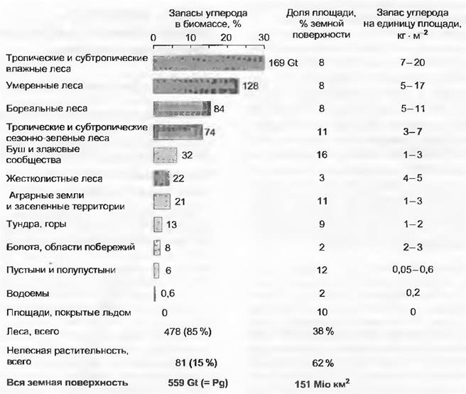
In accordance with the Definitions given in Section 12.5.1.4, biomass does not include dead plant parts. However, in such general statistics, a precise Separation of bio- and necromass is practically impossible. What is referred to here as biomass, following the literature, is actually phytomass (i.e., including necromass). Considering that these tree trunks represent the evolutionary outcome of competition for light and, to some extent, surrounding space ("escape" from herbivores and fires), this means—translated into everyday language—that the predominant share of above-ground biomass surprisingly consists of "advertising costs."

Almost half of all the Earth's forest formations (about 42% of total biomass) are found in the tropics and subtropics. Average biomass stocks in agricultural crops reach approximately 1.6%, while only 0.2% of total biomass resides in the oceans. In forests, most biomass is concentrated above ground (about 80%), whereas in grassland communities it is predominantly subterranean (more than 60%, with extreme values up to 90%). Typically, 60–80% of total root biomass is concentrated in the upper layer of the soil profile down to a depth of 30 cm, though a small fraction of roots generally penetrates the soil to a depth of several meters, except in subpolar vegetation and waterlogged habitats (Table 13.3).

Table 13.3. Total and unit-area root mass in major biomes, along with mean maximum and absolute maximum root penetration depths

According to calculations by R. Jackson and D. Canadell, the Earth's total root mass is about 235 Gt of dry matter, or approximately 140 Gt of carbon. Because this source includes root biomass penetrating deeper soil layers—due to a specific Selection of literature data on roots—which is not reflected in classical tables of the Earth's total biomass (where root mass below 30 cm from the surface is typically ignored), these values appear higher than subsequent estimates (85 Gt dry mass, or about 40 Gt carbon, which would correspondingly increase the global carbon stock from 560 to 600 Gt) (see Figs. 13.38 and 13.39). The discrepancy in area percentages (Fig. 13.38) stems from different formations ordinations.

* Overall, the mean maximum root depth is 7 m for trees, 5 m for shrubs, 2–6 m for herbaceous plants (including grasses), and 2 m for cultivated crops. Lacking additional data, one can assume as a first approximation that these life forms reach the aforementioned depths with the tips of their deepest roots (depths may be shallower in cool, humid regions and deeper in hot, dry ones).

Reserves of dead plant material in certain grassland communities can reach 50–90% of the total plant mass (dead leaves and leaf bases). A similar situation can occur in forests if the physiologically inactive heartwood is regarded as "dead" (in contrast to active sapwood), though this cannot be proven statistically. Dead plant mass in the soil, known as litter, is generally small in grasslands, but amounts to 5–10 t ha^-1 in forests (the lower value for deciduous forests, the upper for coniferous ones), with annual litter production ranging from 4 to 5 t • ha^-1, which is roughly equivalent to annual wood increment.

Once vegetation fully covers the ground, biomass varies without significantly affecting LAI (see 12.5.1.5). Mown meadows and well-stocked beech forests exhibit similar LAI values of around 6. Accordingly, the chlorophyll content per unit of land surface in closed vegetation is globally consistent (2–3 g • m^-2).

The magnitude of biomass reserves tells us nothing about metabolic turnover rates. Although the oceans contain only a minuscule fraction of the Earth's biomass (mainly plankton), these organisms collectively supply nearly as much carbon annually as terrestrial vegetation. This comparison demonstrates that the difference between "pools" and fluxes (metabolic reactions) is crucial for understanding the carbon regime, particularly regarding the CO₂ issues discussed further below (see 13.7.6).

13.7.5.2. Biomass Production

When plants grow, thereby increasing their biomass per unit area over time, we speak of biomass production or, when expressing the rate per unit time, of productivity. Because plant biomass production forms the foundation of the food chain, it is termed primary production. A distinction is made between gross primary production (GPP)—the total amount of biomass synthesized per unit area—and net primary production (NPP), which remains after subtracting current respiration losses (R) within the ecosystem:

These production terms, familiar from economic life and widely used in biology generally, are theoretical concepts and hardly applicable in practice because the magnitude of losses—especially those occurring underground and through respiration—is typically unknown. Estimates of NPP are therefore prone to large errors.

As can be gathered from rough benchmark figures, approximately half of the carbon assimilated by a plant is released during its lifetime as CO₂ via respiration. Another portion typically returns to the atmosphere through microbial decomposition. In a global comparison of forest data, J. Reich and K. Nadelhoffer demonstrated that annual above-ground litter production (70–500 g m^-2 a^-1) corresponds to the release of CO₂ from the soil ("soil respiration"), leading to the conclusion that above-ground and underground production are governed by the same factors.

NPP, the most frequently used metric, has never been empirically determined even approximately using the formula above. Doing so would require knowing the cumulative amount of bound carbon and all respiration losses over the entire observation period. To bypass this, researchers routinely examine The change in biomass reserves (ΔB) between two points in time (g • m^-2 • a^-1). The problem is that a vast amount of produced biomass is lost again during the observation interval. Dead SHOOT parts (V₀) can still be continuously collected and factored into the final calculations (naturally excluding volatile losses such as isoprene — Ex₀); it is much harder to reconstruct the biomass consumed by herbivores and pathogens (C₀), while for underground organs it is utterly impossible to determine biomass losses and consumption (V₀, C₀). In grasslands, more than two-thirds of the biomass is allocated to subterranean organs, and most fine roots are short-lived. Estimates suggest that another 5–10% of assimilates are transferred to mycorrhizal Fungi and retained there briefly, which is similarly unquantifiable. The amount of root exudates released into the rhizosphere (sugars, Amino Acids) remains largely unknown, as do losses of dissolved organic matter (DOM) leaching into percolating water (E_xy) in most cases. Given that NPP determined from biomass changes (ΔB) can be 100% inaccurate, the equation

(V — dead, lost biomass; C — consumed biomass; Ex — export of biomass, both above-ground and underground) is practically unsolvable. NPP data derived from biomass yield (ΔB) would be comparable only if all these loss variables were equal across all ecosystems, which is highly improbable. An additional challenge is the allocation of biomass over the observation period. Because new above-ground structures built from reserves in deep-seated soil organs were not actually produced during the observation period (stored growth), the biomass was merely translocated from bottom to top (at a metabolic cost).

Due to these unknown loss variables, it is more accurate to speak of net phytomass increment rather than NPP, or, as customary in agriculture, of harvested yield. Because of this inaccuracy, NPP values are sometimes cited as NPP. Nearly 46–50% of dry matter consists of carbon units. The average energy content (calorific value) of biomass is 18.1 kJ for terrestrial plants and 19.3–20.6 kJ for oceanic plankton.

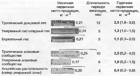
When estimating biomass increments in the Earth's major biomes as a practical approximation of true "productivity," the result depends on the chosen time scale. If the non-productive season in high-latitude regions (winter dormancy) is included—i.e., evaluating biomass increment over a full year regardless of the actual growing season—apparent productivity decreases toward the poles. However, if only active growth periods are compared, productivity is roughly uniform across the Earth as long as water is sufficient. This striking, frequently overlooked result demonstrates how physiological adaptations universally compensate for climatic differences. Latitudinal differences in productivity (let alone regional and local variations in growing conditions) result almost entirely from differences in growing season length; the climatic influence during the season itself is very minor. If monthly averages of the vegetative period are used instead of annual figures, high-altitude plants in temperate zones (the Alps) produce no less biomass than the average tropical rain forest, and Central European beech forests match this performance as well (Fig. 13.39). Under exceptionally favorable growth conditions, such as in intensive agriculture, annual biomass accumulation can exceptionally exceed 5 kg • m^-2.

Fig. 13.39. Biomass "production" in various ecosystems. Annual figures (in bold on the right, including growth dormancy periods in extra-tropical regions) are compared with values recalculated for the average month of the growing season (rectangles on the left), revealing starkly different outcomes (data for humid regions only). This clearly illustrates that global variations in annual biomass accumulation are hardly influenced by temperature conditions during the growing season. Average production data for forests and grasslands do not differ significantly (values in parentheses indicate high regional and local Variability).

The difficulty in extrapolating biomass reserves and increment lies in the fact that extremely labor-intensive analyses are carried out in only a few locations across the globe. Naturally, such studies often target "ideal" and mature stands. Consequently, global biomass is evidently much lower than estimated during the International Biological Program (1968–1974). At that time, the global terrestrial biomass reserve was estimated at 840 Gt of carbon. Newer assessments, conducted on areas with "imperfect" vegetation and bare surfaces, fall within the range of 560–600 Gt of carbon (disregarding the rapid disappearance of tropical forests, estimated at 1–2 Gt of carbon per year, which is counterbalanced by net growth in the temperate zone; see 13.7.6).

Table 13.4. Biomass of a Central European mixed oak-hornbeam forest

Through their living and dead mass, primary producers form the foundation for further matter Processing by consumers and decomposers, i.e., for secondary production. In accordance with food chain dynamics, plant biomass exceeds the mass of secondary producers by hundreds of times. Among consumers, the greatest biomass is held by herbivores, whereas first- and second-order carnivores and, accordingly, first- and second-order parasites—with progressively decreasing zoomass—form the apexes of trophic pyramids across various trophic levels. Table 13.4 and Fig. 13.40 illustrate, by way of example, the distribution of biomass and production values in a Central European mixed oak-hornbeam forest. It is evident here that the trophic pyramid corresponds to the production pyramid, since net primary production reaches values that are an order of magnitude higher (tens to hundreds of times) than those of secondary production, as is also the case in other ecosystems.

Fig. 13.40. Annual solar radiation, as well as Primary and secondary production in a Central European mixed oak-hornbeam forest (cf. Table 13.4)

Figure 13.40 also shows that consumers account for only an insignificant share of secondary production, because only about 2% of the plant primary production in the oak-hornbeam forest is directly consumed by herbivores (in other terrestrial biocenoses scarcely more than 15%, averaging about 7%). At the same time, nearly 25% of production is accumulated annually as dead organic matter in solid form (detritus: leaf litter, humus, etc.) or in soil solutions (e.g., humolignin acids). This quantitatively important compartment of the ecosystem corresponds to the high significance and productivity of saprotrophic and mineralizing decomposers (see 9.1.1, Box 11.4); their share in secondary production is 95%.

Despite the unreliability of the aforementioned database, global comparisons of NPP estimates are highly illustrative (Fig. 13.41). Although oceans account for only 0.2% of the global biomass reserve, due to their vast expanse—covering 70% of the Earth's surface—they exhibit NPP values almost as high as those of the entire landmass. Productivity, however, is concentrated in nutrient-rich areas and regions, i.e., coastal zones with upwelling deep cold waters. The open-ocean tropical and subtropical Regions of the world are productive deserts (white areas on the map). Notably, maximum natural productivity in the sea (specific coastal zones) and on land can be very similar, namely 2,000–3,000 g • m^-2 • yr^-1 (point peak NPP values reach up to 6,000 g • m^-2 in land-sea transitional zones, almost matching tropical and subtropical swamps). On land, the mean annual NPP of closed-canopy vegetation varies by latitude and water availability from 200 (subpolar regions) to 2,500 g • m^-2 (tropical rain forests, all biomass given in absolute dry weight). Productivity in temperate forests is about 1,000–1,500 g • m^-2 (see Fig. 13.39). Nearly 25% of the Earth's surface (about 33 million km²) exhibits an annual NPP of no more than 500 g • m^-2. For cultivated plants, the upper limit can approach 7,000 g • m^-2 (irrigated intensive sugarcane crops). Algal cultures (e.g., Scenedesmus) can yield 10,000 g • m^-2 of biomass under laboratory conditions, but their Practical Application remains challenging.

Fig. 13.41. Net primary production of the biosphere. Data are given in grams of dry matter per 1 m² per year for land and oceans

According to recent estimates, global NPP amounts to approximately 210–250 billion t of biomass, or 100–120 billion t of carbon (46–50% of biomass), of which 50–60 billion t of carbon each are produced in the ocean and on land (1 billion t = 1 Gt = 1 Pg = 10¹⁵ g). On land, approximately half of the NPP is concentrated in the tropics. The average residence time of carbon is 22 years on land, compared to roughly a week in the ocean (plankton <5 µm; high surface-to-volume ratio).

13.7.5.3. Net Ecosystem and Biosphere Production

Net ecosystem production, NEP (net ecosystem production), is a production parameter far better defined than NPP and measurable with a much closer approximation to reality. NEP represents the net carbon balance of an ecosystem—that is, the difference between carbon uptake and release—regardless of where and how carbon is periodically bound within the system.

NEP is most reliably determined over long time intervals (at least one year) and large spatial scales (>1 ha). The baseline data are obtained by measuring CO₂ fluxes (influx and efflux) using meteorological Methods (measurement towers positioned above a homogeneous, flat landscape plot). The so-called "eddy covariance" method employs a three-dimensional ultrasonic anemometer to measure vertical bulk fluxes of air parcels and instantly couples them with an open-path infrared gas analyzer that measures CO₂ concentrations with very high temporal resolution. The challenge in measuring NEP with this method lies in capturing a very small net difference between exceptionally large fluxes. Demonstrating that NEP is non-zero requires extremely high measurement accuracy. Selecting "ideal" homogeneous stands generally leads to an overestimation of net fluxes at the whole-landscape level. Export of carbon in forms other than CO₂ is not captured by standard NEP measurement Procedures.

Of great significance for ecosystem functioning is not only the flux of matter and energy between the system itself and its surroundings, but also the allocation and intensity of fluxes within the system. The annual energy flux of a subtropical spring-fed lake (Fig. 13.42) carries very little phytomass (yet Supports numerous generations of planktonic Algae) and illustrates how primary production energy is distributed along the trophic chains of the ecosystem.

Fig. 13.42. Energy flux through a natural plankton ecosystem (Silver Springs subtropical spring-fed lake, Florida)

Input and output values are given in kJ • m^-2 • yr^-1. Compartments from left to right: primary producers, consumers (herbivores — PFLF and first- and second-order carnivores — FF), and decomposers (ZS)

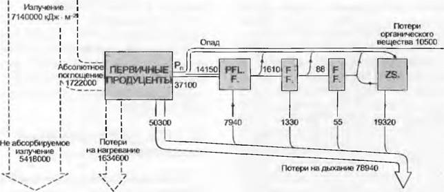
In terrestrial biocenoses, particularly in long-established forests, the cycling of matter and energy proceeds significantly slower relative to phytomass. Although nearly a quarter of the incident solar radiation is absorbed in this spring-fed lake, the relatively dense phytoplankton can ultimately utilize only 1.2% of the total radiation for gross production, despite the absence of a winter dormancy period. Following relatively high respiration losses (70%), only 20% remains for consumers and decomposers.

The more mature an ecosystem is, the closer its NEP approaches zero. Soil carbon reserves (in most cases 10–20 kg • m^-2) play a crucial role in this carbon balance. In the humid tropics, they often account for no more than 10–20%, in boreal coniferous forests for 60–70%, and in tundra for over 90% of the total ecosystem carbon. When soil humus initially decomposes rapidly in fast-growing forest plantations (due to drainage, Fertilization, liming), NEP can become negative despite a very positive NPP. In young ecosystems, NEP is mostly positive; in mature ones, it approaches zero; and in old, degrading ones, it is negative. Only by capturing all these developmental stages present across a landscape (forest region) can one determine whether net carbon sequestration is occurring within the ecosystem or not.

A forest in the regeneration stage, as well as a mature forest prior to logging, consistently exhibit positive NEP values. The subsequent fate of the trees dictates the long-term trajectory of NEP. If the next generation of trees develops within an ecosystem enriched with coarse and fine humus following the decay of dead wood, NEP can remain positive for centuries. If commercial timber is harvested and eventually recycled (paper, waste recovery, incineration, decomposition), the calculated NEP once again approaches zero. Wooden structures, for instance, represent an intermediate carbon pool.

Thus, forming an objective judgment on the landscape carbon balance transcends the boundaries of a single ecosystem; consequently, for very large scales and extended time frames, NEP is replaced by NBP — net biome production. NBP encompasses landscape-level processes such as fires, windthrows, and insect outbreaks, accounts for all vegetation development stages—including internal canopy gaps—and incorporates the consequences of human activity as well. Across most of the world, NBP is currently negative, meaning that biomes are losing net carbon (due to deforestation, intensive soil tillage, and the expansion of densely populated and industrial areas), although ecosystems with positive NBP still exist in some regions.

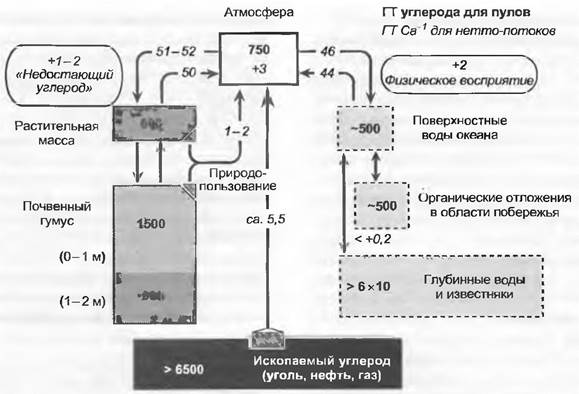
The next step leads to the biosphere as a whole. Its carbon balance is roughly in equilibrium, as the Earth's ecosystems bind on average as much carbon as they release. The ongoing deforestation in the tropics releases 1–2 Gt of carbon into the atmosphere annually, while as yet insufficiently understood biotic sinks sequester another 1–2 Gt of C—a phenomenon presumed to be driven by The Fertilization Effect of elevated atmospheric CO₂ levels and the intensification of land use in various parts of North America and Europe (secondary and lightly managed forests). The current rise in atmospheric carbon is driven by anthropogenic release of fossil carbon reserves amounting to 5–6 Gt annually; a portion of this dissolves in sea water, leaving "only" nearly 3 Gt of additional carbon in the atmosphere each year. This increases the atmospheric carbon pool (in the form of CO₂) from its current value of 750 Gt by 0.4% annually, or nearly 1 ppm (current value 370 ppm). Continuation of this trend will lead to a doubling of overall CO₂ levels by the end of the 21st century compared to the pre-industrial era (see 13.7.6). Pools and fluxes integrated into the global carbon cycle, including contemporary anthropogenic fluxes, are illustrated in Fig. 13.43.

Fig. 13.43. Global carbon cycle in an environment subject to human influence (anthropogenic C sources are shaded). Box sizes reflect the magnitude of carbon reservoirs. Only about 40% of the released fossil carbon currently remains in the atmosphere; the remainder dissolves in the ocean and is sequestered in terrestrial ecosystems (1–2 GtC of "missing carbon"). This figure roughly corresponds to the annual carbon release resulting from deforestation. Large carbon pools in the deep ocean and in carbonate rocks influence atmospheric CO₂ concentrations only over extremely long time scales (deep ocean >200 years, significant interactions with carbonate geochemistry >1,000 years)

13.7.6. Biological Aspects of the CO₂ Problem

Because fossil carbon sources—which largely began to form more than 100 million years ago and developed over millions of years—have been pumped into the atmosphere by humans as CO₂ within a span of roughly 200 years (roughly speaking, from 1910 to 2100, when easily accessible reserves may be exhausted), vegetation faces an entirely novel situation. The biosphere is receiving a new "diet," as it were, overnight in geological terms. Since CO₂ is the material basis of photosynthesis, upon which all life on Earth depends (aside from a few chemoautotrophic bacterial species), the CO₂ problem has become central to ecological botany. The possibility that atmospheric CO₂ enrichment is also linked to climate (the so-called greenhouse effect) and could consequently exert an indirect influence on plants is not discussed here; the focus is exclusively on the direct impact on plants and ecosystems.

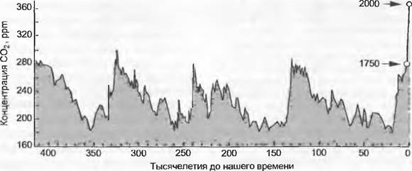
It is believed that atmospheric CO₂ levels at the beginning of the Carboniferous period were around 2,000 – 3,000 ppm, but then dropped very rapidly to 300 – 500 ppm, which is close to modern levels, and that the lowest values occurred during the Permian period. It has been reliably established that during the Cretaceous, CO₂ levels were initially very low (about 300 ppm), which explains the first mass proliferation of C₄-type plants. The Mechanism of CO₂ concentration by C₄ plants operates only at very low CO₂ levels, giving them an advantage over C₃-type plants. Using ice cores from Antarctica, the COMPOSITION OF THE atmosphere has been documented over the past 0.4 million years (by analyzing air bubbles trapped in the ice). As Fig. 13.44 shows, the CO₂ concentration fluctuated during this period within the range of 180 — 290 ppm. Maxima correspond to warm periods, and minima to glacial peaks. Since 1800, i.e., the onset of coal heating, the curve has exceeded this range and by roughly 1900 rose so steeply that the air now contains 30% more CO₂ than when most park trees were originally planted. Almost all currently existing plant species emerged in ice-free regions during a time when the CO₂ level was 180 ppm (otherwise they would simply have gone extinct; the last time CO₂ concentration was this low was approximately 20,000 years ago). Around 1990, they experienced a doubling of this value (reaching 370 ppm in 2000). Unless a global collapse of the world economy occurs, the CO₂ concentration will double again over the next 100 years.

Fig. 13.44. Atmospheric CO2 concentration over the past 0.4 million years based on the analysis of air bubbles in the Antarctic ice sheet (Vostok station core drilling)

The starting point for all discussions regarding the biological consequences of rising CO₂ lies in the response curve of net photosynthesis to CO₂ concentrations (Fig. 13.45, see 6.5.11.2). It demonstrates that C₃ plants can exist at even higher concentrations than today and achieve higher rates of photosynthesis. Of course, such curves are essentially "snapshots of the moment," which merely prove that under current Rubisco supply conditions and without limitation from assimilate deposition, the carboxylation process is not yet saturated with CO₂. As explained in sections 13.7.2 and 13.7.3, growth acceleration depends on many other factors, and only when sink limitation is absent can CO₂ concentration be classified as a growth stimulant.

Crop yield increases in greenhouse horticulture amount to roughly 30% per season when plants are provided with a CO₂ level of 600 ppm or more—a practice already utilized in German and Dutch greenhouses prior to World War II. Well-fertilized and irrigated wheat fields in Arizona produced 14% more grain when cultivated at a CO₂ level of about 600 ppm. These figures should be viewed in the context that wheat yields have already increased by 300 – 500% over the past 100 years thanks to new varieties and optimal management.

When all resources other than CO₂ act as growth-limiting factors—which is almost always the case under natural conditions—three possibilities for long-term response remain:

✵ reduction of photosynthetic capacity (less Rubisco and thus less nitrogen per leaf area, or fewer leaves, i.e., lower LAR, see 13.7.3);

✵ higher carbon export (e.g., more rapid fine-root turnover, root exudation, export to mycorrhizae, emission of isoprenes);

✵ enhanced growth via nutrient dilution, particularly N, i.e., the production of biomass with a higher C/N ratio.

All three pathways generally run in parallel. Typically, a reduction in photosynthetic capacity occurs, but almost never completely, so that under elevated CO₂ conditions, more carbon is almost always fixed per unit of leaf area (Fig. 13.45).

Fig. 13.45. Down-Regulation of the photosynthesis-CO₂ response curve under prolonged exposure to increasing CO₂ content (down-regulation — dashed curve) depends on growth conditions (sink activity for assimilates) and plant age. Point NA denotes the increase in net photosynthesis when CO₂ concentration is raised to 600 ppm without such regulation; D represents the remaining net gain after regulation

Numerous experiments show that carbon export is enhanced under elevated CO₂. It has been observed that higher levels of soluble carbohydrates in the rhizosphere lead to increased nitrogen immobilization by soil microorganisms, which can result in symptoms of nitrogen deficiency. An increased C/N ratio has been observed almost universally, particularly in leaves. In most cases, the total content of non-structural carbohydrates increases (e.g., starch, sugar; non-structural carbohydrates — NSC). Along with a decrease in protein content (N) and an increase in NSC content (C), nutritional quality also changes. It has been proven for herbivores that this negatively affects their GROWTH AND REPRODUCTION.

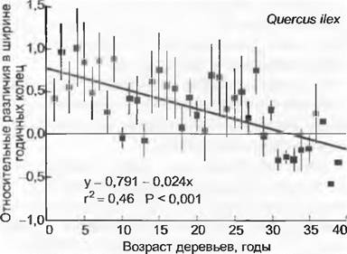
Biomass accumulation in natural vegetation (with nearly all data derived from grassland communities) is usually very slight (less than 15% under a simulated doubling of CO₂ concentration) or even zero. For natural forests (representing 85% of global biomass stock), data are lacking, but the response of holm oaks growing at the margin of a natural CO₂ spring in Tuscany provides initial evidence of a potential reaction: growth stimulation during the early juvenile phase of development under adequate light and nutrient supply. As age increases, the response diminishes until the effect is reduced to zero (Fig. 13.46). This could signify a certain acceleration of The life cycle. A higher biomass stock per unit of land area is not necessarily linked to this. A considerable number of CO₂ experiments with tree seedlings have demonstrated this only at very early stages. Most species respond positively to CO₂, but in a highly species-specific manner, with differences depending on the simultaneous supply of light and nutrients, rendering definitive generalizations impossible.

Fig. 13.46. Effect of elevated CO₂ content on the long-term growth of trees in the vicinity of a geological CO₂ spring in Tuscany (Rapolano). Through tree-ring Analysis of the holm oak (Quercus ilex), it can be observed that trees in early developmental phases near the spring grew markedly faster compared to more distant control trees (the figure shows the difference in increment relative to trees away from the spring). At approximately 30 years of age, the signal disappears (experiment/control index is zero; solid line). Dispersion bands indicate the standard variability in each case for 10 trees. Carbon (¹⁴C) analysis of the tree-ring wood established that trees exposed to the spring actually experienced a CO₂ concentration twice as high as that of the controls (geological CO₂ is devoid of ¹⁴C; by mixing it with normal air, the average CO₂ concentration experienced by the trees can be reconstructed)

Across all plant responses to CO₂, it has been established that different species react very diversely. In some instances, it has even been observed that different genotypes of the same species do not respond identically. This implies that the CO₂ problem must in any case be viewed as a biodiversity issue of a unique kind. CO₂ supply influences competitive relationships among species. It is widely agreed that this factor affects species composition structure on a global scale.

Aside from the Direct impact of CO₂ on photosynthesis and subsequent assimilate utilization, there is also an indirect effect of CO₂ mediated through the water regime. Stomata frequently respond to increased CO₂ concentration by narrowing the stomatal pore (see 8.3.2.5). This response depends on atmospheric and soil humidity; it is not equally strong in all species, and in trees, it is more pronounced at the seedling stage than in mature specimens. In grassland communities, this stomatal response leads to a slower decline in soil moisture during precipitation-poor periods, which is the primary cause of increased biomass accumulation. A large portion of the phenomena occurring in natural grassland vegetation can be attributed to this indirect effect. In dry years, this effect manifests more strongly than in wet years (Fig. 13.47). It is hypothesized that The Effect of slowed moisture depletion in a CO₂-enriched environment will become reality provided that evaporation conditions remain unchanged relative to the present day.

Anthropogenic CO₂ emissions currently amount to nearly 6 Gt C • a^-1 and will continue to rise, meaning that vegetation will be unable to sequester the incoming surplus over the next 100 years or more. It is far more likely that land-use carbon will be transferred to the atmosphere. Already today, even on the steep slope of the photosynthesis-CO₂ response curve when CO₂ exceeds pre-industrial levels by 30%, the maximum net fixation is only 2 Gt (even if the estimated terrestrial carbon uptake (see Fig. 13.43) is attributed exclusively to the CO₂ fertilization effect, which is likely an overestimate)—this is a surprisingly small fraction of the global net primary production of terrestrial vegetation, which is about 60 Gt C • a^-1. Due to stoichiometric P and N fixation and other constraints, the relative effect of increasing CO₂ concentration is significantly diminished.

Fig. 13.47. Effect of elevated CO₂ content in a tallgrass prairie plot. Only in dry years does elevated CO₂ concentration stimulate biomass accumulation; this is a result of The impact of CO₂ on stomata, Transpiration, and consequently soil moisture (600 vs. 360 ppm in large open-top chambers).

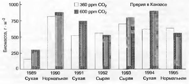
Biomanagement aimed at enhancing plant carbon sequestration is rational and ecologically beneficial, but one should harbor no illusions that its absolute values are directly coupled to carbon emissions. Only a substantial expansion of forest areas could contribute to long-term carbon sequestration in biomass. At present, however, forest areas are undergoing massive reduction. Afforestation of cleared land gradually compensates for these losses, but yields no net increase until previous conditions are fully restored—a process subject to a 100- to 200-year time lag. Old-growth trees contain substantially more carbon than young ones; therefore, replacing mature stands with young ones always (!) represents a carbon loss. It must be borne in mind that in the long-term carbon balance, the decisive factor is not the turnover rate, but the magnitude of the total pools (the mean residence time of carbon in the landscape). Fast-growing forest plantations do not contribute to repaying a region's carbon "debt," although they can serve as a valuable source of renewable resources (substituting for fossil carbon sources). To make the orders of magnitude of this substitution potential clear, Fig. 13.48 illustrates how much fossil carbon could theoretically be replaced by biomass if all (!) harvested wood annually in Germany, Austria, or Switzerland were put to this use (other uses of wood and the technical application of substitutes are not assumed). The figures indicate that the problem cannot be solved either in this manner or through the establishment of dedicated biomass plantations, as the biomass accounts for only a few percent of fossil carbon. This does not mean that utilizing biomass instead of fossil carbon is undesirable or devoid of ecological and economic benefits. No biomass effect can even remotely approach the mitigation potential of even small (less than 5%) conservation quotas in fuel consumption, whereas technically feasible savings—combined with those resulting from behavioral changes—can exceed 50% without any significant reduction in living standards. Therefore, one must not lose sight of the orders of magnitude when relying on the role of plants to solve the problem.

Fig. 13.48. Substitution potential of fossil carbon by biological carbon sources. The annual production of fossil carbon is compared with its content in all timber harvested by the national forestry sector or, alternatively, the mass of carbon obtained from biomass plantations (e.g., Chinese reed) on 10% of current arable land