PLANT BIOPHYSICS - Y. I. Posudin - 2004

II. TRANSPORT PROCESSES IN THE SOIL-PLANT-ATMOSPHERE SYSTEM

6. MASS TRANSPORT

6.8. WATER AND SOLUTE FLOWS IN PLANTS

Class="center">6.8.1. Water Flow in The Cell

The difference in water potentials ΔΨ_в across a membrane or membranes bounding the volume of water flow J_k serves as the driving force that maintains this flow:

where J_в is the volume flux of water flowing through a unit surface area per unit time (м³/м²·с = м·с^-1), L_в is the water permeability coefficient (м·с^-1·МПа^-1), and Ψ^е_в and Ψ^і_в are the water potentials of the external and internal solutions, respectively.

Considering water flow through several (j) Cells connected in series, the transport process is described by the following equation:

Let us calculate The water potential difference required to drive the water flow observed in the freshwater Algae Nitella and Chara, whose internodal cells have a length of l = 10 см and a diameter of r = 1 мм. The water permeability coefficient for such cells is L_в = 10^-6 м·с^-1·МПа^-1. Water enters from the external medium through the lateral surface of the cells, the area of which is The volume of the cylinder formed by the cell is Assuming that the Cell Growth Rate (and the corresponding increase in water content) is 1 % of the cell volume per day, we estimate the total volume of water flow over a day as Hence, The rate of water influx per unit of lateral cell surface area per unit time is:

Thus, we find the water potential difference ΔΨ_в from equation (6.22).

The algae under consideration inhabit pond water, which is a dilute aqueous solution with a WATER POTENTIAL OF -0.007 MPa. Therefore, the water potential inside the cell must be 3·10^-5 MPa lower than the water potential of the external environment to ensure water influx into the cell.

6.8.2. Solute Flow in the Cell

Let us consider the coupling of two flows across a membrane—water and solute. The membrane is permeable to both water and the solute. The driving force for both flows is the gradient of chemical potential. Using equation (6.22), we can represent each flow as a linear combination of driving forces:

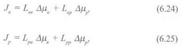
where the subscripts в and р refer to water and solute, respectively.

It is evident from the equations that each flow depends on both chemical potentials. Since, according to Onsager's reciprocity principle for phenomenological coefficients, L_вр = L_рв, only three phenomenological coefficients need to be known to describe the dependence of the two flows on the two driving forces.

The difference in chemical potentials can be expressed in terms of osmotic and hydrostatic pressures. Using equation (6.13), we find the difference in chemical potentials:

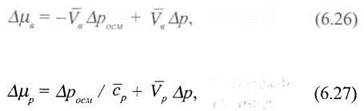
where is the average solute concentration.

Thus, the changes in chemical potentials Δμ_в and Δμ_р, which act as the driving forces of the process, are expressed as Functions of the same pressure differences Δр_осм and Δр.

6.8.3. Water Flow in the Soil-Plant-Atmosphere System

Water serves as the primary medium for the biochemical and biophysical processes that drive plant METABOLISM. It dissolves sugars and minerals for long-distance transport throughout the plant, acts as a reactant in Photosynthesis, maintains the necessary turgor pressure within cells, and regulates plant Temperature via Transpiration. Additionally, water vapor lowers the density of the surrounding air, thereby facilitating air Circulation within the plant canopy. Water moves in a continuous stream from the soil, through The ROOT System and stem, into the leaves, and eventually out into the atmosphere via Stomata. While continuous, this flow is heterogeneous, as water sequentially moves through the soil to the roots, is absorbed by the root system, is transported through xylem vessels, diffuses through intercellular spaces and stomata, and finally escapes into the atmosphere as water vapor. The driving forces governing this water movement are: a pressure gradient in the soil, a water potential gradient in the root system, a pressure gradient for long-distance transport through the xylem, and a water vapor concentration gradient during transpiration (Fig. 6.14).

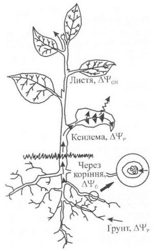
Fig. 6.14. Main driving forces governing Water movement through the soil-plant-atmosphere continuum: pressure gradient in the soil, water potential gradient in the root system, pressure gradient for long-distance transport through the xylem, and water vapor concentration gradient during transpiration.

The amount of water lost by a plant through transpiration equals the amount absorbed by its root system. Consequently, the water flux within a plant can be considered steady-state. Under these conditions, electrical circuit analogies can be applied to water transport, treating the water flux as analogous to an electric current, which is equal to The ratio of the water potential difference ΔΨ to the hydraulic resistance r:

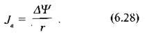
Applying this equation to the soil-plant-atmosphere continuum, we obtain:

where Ψ_г is the soil water potential, Ψ_к is the root water potential, Ψ_л is the leaf water potential, Ψ_а is the atmospheric water potential, r_г-к is the resistance to water flow from the soil into the root system, r_p is the internal plant resistance, r_n is the stomatal resistance, and r_a is the atmospheric (boundary layer) resistance.

The first two ratios correspond to liquid-phase fluxes, whereas the last one represents the gas-phase flux. Typical water potential differences observed across various segments of the soil-plant-atmosphere continuum are as follows [Cruiziat, 1987]:

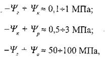
where Ψ_г, Ψ_к, Ψ_о, Ψ_л, and Ψ_а represent the water potentials of the soil, roots, whole plant, leaves, and atmospheric water vapor, respectively.

The decrease in water potential along the water transport pathway in the soil-plant-atmosphere continuum is illustrated in Fig. 6.15. The water potential of moist soil, roots, and stems remains close to zero, corresponding to its maximum value (curve 1). Leaves exhibit a lower water potential, which is nevertheless high enough to prevent wilting, keeping the stomata open under these conditions. A drop in soil water potential (curve 2) induces a corresponding decrease in water flux and leaf water potential, which triggers stomatal closure.

The water potential of moist soil consists of the osmotic potential and the pressure potential. The osmotic potential of soil water is sufficiently small (-0.02 MPa) that it can be neglected, although in brackish soils the osmotic potential increases to -0.2 MPa. The hydrostatic pressure of moist soil is close to zero. Soil drying causes water to be removed from the spaces between soil particles, leading to The formation of concave surfaces, or menisci. The tensile state of the liquid surface layer is called surface tension, and the forces responsible for contracting the surface film of a liquid are called surface tension forces. Water is characterized by an exceptionally high surface tension: at 20 °C, the surface tension at the air-water interface is 72.8·10^-3 N·m^-1. If the liquid surface is curved, it exerts an additional pressure on the liquid due to surface tension forces. For a spherically curved surface, this additional pressure is determined by the Laplace formula:

where σ is the surface tension coefficient and R is the radius of curvature of the liquid surface. The additional pressure is taken with a plus sign if the surface is convex, and with a minus sign if the surface is concave. Consequently, a negative additional pressure arises at the water-air interface: Ψ_p = -2σ/R, where R is the radius of the meniscus.

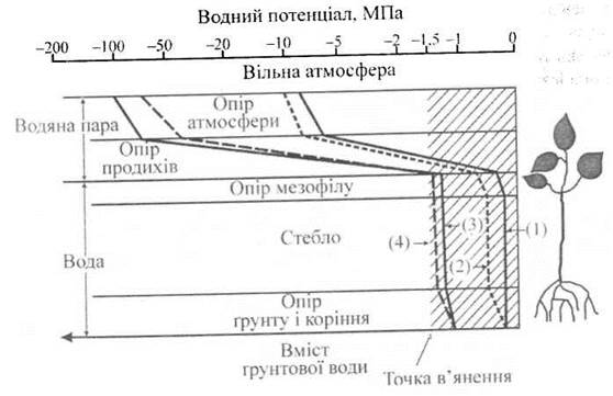
Fig. 6.15. Decrease in water potential during water transport within the soil-plant-atmosphere continuum.

In the previous sections, it was noted that the main Mechanisms of water transport are molecular diffusion and bulk flow. Over long distances, water transport is governed by bulk flow driven by a pressure gradient. Due to water absorption by the plant, soil water is depleted, leading to a decrease in the water pressure potential Ψ_p near The surface of the root system. This results in the formation of a pressure gradient along which water from other soil areas moves through soil pores. The rate of water flow depends not only on the magnitude of the pressure gradient but also on the hydraulic conductivity of the soil, which varies with soil type (sand, for example, has a high hydraulic conductivity, unlike clay). In excessively dry soils, the water potential Ψ can drop to a critical threshold known as the wilting point. Under such conditions, the plant is unable to restore its turgor pressure and wilts.

6.8.4. Root System

The absorption of water and mineral nutrients from the soil by a plant is carried out through the root system. Reliable contact between the roots and the soil is ensured by A large number of roots and root hairs. For example, consider the parameters of the root system of a four-month-old rye plant [Polevoy, 1989]: average number of roots, 1.38 · 10⁷; total surface area of the root system, 232 m²; number of root hairs, 1.4 · 10¹⁰; total surface area of roots and root hairs, 631 m². Notably, the total surface area of the root hairs can account for up to 60% of the total surface area of the root system.

During its passage through the root system, water absorbed by a root Hair crosses the epidermis and is transported either via the symplastic pathway—through the Cytoplasm via plasmodesmata, which are microscopic cytoplasmic strands connecting the protoplasts of adjacent cells—or via the apoplastic pathway—through the cell walls (Fig. 6.16).

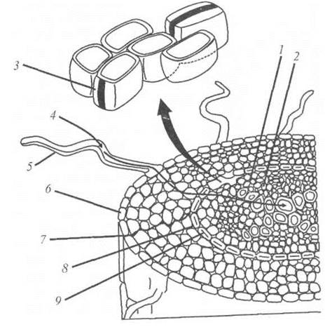
Fig. 6.16. Pathways of water transport through the root system via the symplastic or apoplastic route: 1 - phloem, 2 - xylem, 3 - Casparian strip, 4 - cellular pathway, 5 - root hair, 6 - epidermis, 7 - apoplastic pathway, 8 - endodermis, 9 - Casparian strip.

There is a hypothesis [Fensom, 1975; Spanner, 1975] suggesting the possibility of substance transport through the root system via electroosmosis—the movement of liquid along capillary walls, capillary systems, or porous plugs under the Influence of External electric fields. In a macroscopic homogeneous system, water is insensitive to these fields due to its electroneutrality. At the boundary between the Capillary Wall and the liquid, an electrical double layer is formed, consisting of fixed charges adsorbed by the wall and mobile charges located within the liquid. These mobile charges contribute to the generation of an electric field at the sieve plates. The velocity of moving electrical charges is determined by the expression [Ksenzhek, Volkov, 1998]:

where ε is the dielectric permittivity of the medium (80 for water), ε_{д —} is the vacuum permittivity (8.85 · 10^-12 C·V^-1·m^-1), C is the electrokinetic potential, which represents the potential difference between the fixed and mobile charges, ranging from a few units to tens of millivolts, η is the viscosity, and E is the electric field strength (V·m^-2).

The velocity of the electroosmotic flow is low: for typical values of ξ = 20 mV and E = 10⁴ V·m^-1, the velocity is V = 1.4 · 10² cm·s^-1. Since this velocity is independent of the capillary radius, it can be assumed that this mechanism plays a certain role in small-diameter capillaries. There is evidence [Dainty, 1963] indicating the possibility of a pressure gradient generation of about 1 MPa in the root system at a potential difference of 10 mV.

6.8.5. Xylem

The system responsible for supplying water and mineral nutrients from the soil to the upper PARTS OF THE plant is called the xylem. This tissue consists of conductive elements—tracheids, fibers, and vessel elements—that form long rows along longitudinally arranged cells. The diameters of xylem conductive elements range from 10 to 500 µm for various plant species, and their length can vary from a few hundred micrometers to two meters or more. Because these conductive elements lack protoplasts and cell walls, the resistance to the passage of water and solutions through them is very low. A simplified diagram of a xylem conductive element is shown in Fig. 6.17, a.

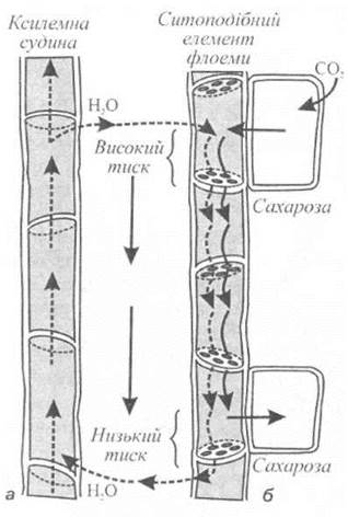
Fig. 6.17. Simplified view of plant conductive elements: a - xylem; b - phloem.

6.8.6. Mechanisms of Xylem Transport

If one end of a narrow tube (capillary) is placed into a liquid, the curvature of the liquid surface (meniscus) becomes significant due to the wetting or non-wetting of the capillary walls by the liquid, resulting in a considerable additional pressure above the surface. The attraction between liquid molecules is called cohesion, whereas the attraction between the liquid and a solid body (the capillary walls) is called adhesion. When the interaction between the liquid and the wall is strong, wetting of the wall by the liquid occurs; conversely, when the intermolecular cohesive forces within the liquid significantly exceed the adhesion between the liquid and the wall, non-wetting takes place. Let us consider a capillary immersed in a wetting liquid. The attractive forces arising between the molecules of the liquid and the capillary cause the liquid to rise along the capillary wall, which leads to a curvature of the liquid surface and the formation of negative pressure. As a result, the liquid rises up the capillary until the hydrostatic pressure balances the additional pressure. The equilibrium condition can be described by the following expression:

where ρ is the liquid density, R is the radius of curvature of the meniscus, g is the acceleration due to gravity, and h is the height to which the liquid rises. From this, the height of the liquid rise can be determined:

where r = Rcosθ is the radius of the capillary, and θ is the contact angle (Fig. 6.18).

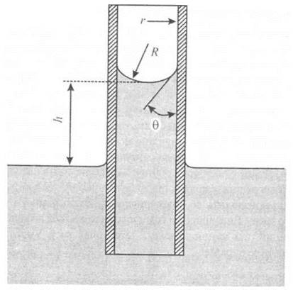
Fig. 6.18. Quantities required to analyze capillary water rise.

Let us consider a specific example of a xylem vessel with a radius of 20 µm: according to formula (6.32), water in the vessel will rise to a height of:

Thus, the additional pressure in xylem vessels is insufficient to drive liquid ascent in plants taller than one meter. Over larger distances, water transport is governed by bulk flow driven by a pressure gradient.

Quantitatively, this volumetric water flow J for cylindrical tubes, such as xylem cells of radius r, is described by Poiseuille's equation:

where η is the viscosity of the liquid, and is the pressure gradient. As can be seen from the equation, the volumetric flow rate strongly depends on the tube radius: doubling the radius increases the volumetric water flow rate by a factor of 2⁴ = 16. Thus, pressure-gradient-driven bulk water flow is the dominant mechanism for long-distance water transport.

Let us apply Poiseuille's equation to estimate the volumetric flow rate of water per unit area (S = nr²) of a xylem vessel, which in this case is determined by the expression:

If the average water flow in the xylem is 10^-3 m·s^-1, the water viscosity coefficient is η = 10^-3 Pa·s, and the xylem radius is r = 20 µm = 2·10⁵ m, then the pressure gradient satisfying equation (6.33) will be = -2·10⁴ N·m³ = -2·10⁴ Pa·m^-1.

The change in gravitational potential per meter of height is (as established in previous sections) ρgh/h = 10⁴ Pa = 10^-2 MPa. In other words, the pressure gradient is capable of overcoming gravity and sustaining the upward Movement of water in the xylem.

6.8.7. Phloem

During photosynthesis, light energy is converted into chemical energy, accompanied by the synthesis of CARBOHYDRATES from carbon dioxide. Although a small amount of carbon compounds, or photoassimilates, is used to support Leaf Growth and metabolic processes, the bulk is exported to non-photosynthetic Organs and Tissues. The long-distance transport of photoassimilates is referred to as translocation. The distribution of most organic substances (primarily photoassimilates) throughout the plant is carried out by the phloem, the plant's second Vascular System. The phloem is a complex tissue composed of several cell types. However, unlike the xylem, the conducting elements of the phloem retain their protoplasts (Fig. 6.17, b). These conducting elements are called sieve cells or sieve tube elements. Connected end-to-end into continuous chains, they facilitate The transport of organic solutes. Dissolved substances move through the phloem: photosynthetic products travel from the leaves to the root system, while sugars can also move in the opposite direction, from the root system to the apex of the plant.

6.8.8. Mechanisms of Phloem Translocation

Any theory attempting to explain the mechanisms of photoassimilate and organic solute translocation via the phloem must account for and elucidate The Structure of phloem sieve elements, the high translocation velocity over long distances (50—250 cm·h^-1), the simultaneous bidirectional Transport of substances, the initial process of assimilates transfer from leaf mesophyll cells to phloem sieve elements (phloem loading), the Transport of Assimilates through the sieve elements, and their ultimate transfer from the sieve elements into the cells of storage organs (phloem unloading).

The pressure-flow hypothesis [Münch, 1930] is widely considered the most plausible. It is based on the mass flow of dissolved solutes from source to sink driven by a hydrostatic (turgor) pressure gradient within the sieve elements (see Fig. 6.17). Phloem loading occurs as sugars are transported from the mesophyll through minor Veins, the midrib, and the petiole into the phloem sieve elements. An increase in solute concentration within these elements leads to a decrease in water potential and a corresponding osmotic influx of water from the adjacent xylem. Consequently, hydrostatic (turgor) pressure rises at this source end of the phloem. Conversely, at the sink end, sugars depart the phloem and water returns to the xylem, lowering the pressure. This establishes a continuous pressure gradient along the phloem that drives the mass flow of liquid from leaves to roots, a process described by Poiseuille's law. This hypothesis is supported by experimental measurements of hydrostatic pressure in sieve elements, which reach values of 2·10⁶ Pa [Nobel, 1973].

Another hypothesis [Fensom, 1975; Spanner, 1975] proposes the involvement of electroosmosis in phloem transport (see Section 6.8.4 "Root System"). It suggests that the driving force for the movement of sugars from one sieve tube to another through pores is K⁺ ion transport, accompanied by the generation of electrical fields across each sieve plate. Several other hypotheses have been proposed to explain assimilate transport mechanisms in sieve elements—such as protoplasmic streaming, peristaltic contractions of cell walls, microelectrokinetic transport, surface-active movement, and others—though they remain insufficiently convincing [Lüttge, Higinbotham, 1984].