PLANT BIOPHYSICS - Y. I. Posudin - 2004

II. TRANSPORT PROCESSES IN THE SOIL-PLANT-ATMOSPHERE SYSTEM

6. MASS TRANSPORT

6.7. MEASUREMENT OF WATER POTENTIAL AND ITS COMPONENTS

Class="center">6.7.1. Tissue Weight Change Method

The Water potential of plant tissue can be determined by establishing equilibrium between the osmotic potential of a solution and the WATER POTENTIAL OF the tissue. To do this, a pre-weighed tissue sample is immersed in a container with a solution of known osmotic potential. If the osmotic potential of the solution is more negative than the water potential of the tissue, water will leave the tissue, resulting in a loss of weight. Conversely, if the osmotic potential of the solution is less negative than the tissue's water potential, water will enter the tissue, increasing its weight. The solution that causes neither a loss nor a gain in weight is considered equivalent to the water potential of the tissue.

In practice, the measurement Procedure (Fig. 6.2) involves preparing tissue samples of identical size and mass, which are then immersed in a solution of known molality (recall that the number of moles per liter of solution is termed molarity, whereas per kilogram of solvent it is molality). To prevent any change in the concentration of the aqueous solution during the measurement, substances that are not absorbed by the tissue (such as sorbitol, mannitol, or polyethylene glycol) are used. After a sufficient period of time, equilibrium is established between the tissue and the solution; the tissue is then carefully blotted to remove residual solution and weighed again. A graph of weight change versus solution concentration is plotted (Fig. 6.3). Using the van 't Hoff equation, the osmotic potential—and consequently the water potential—is determined.

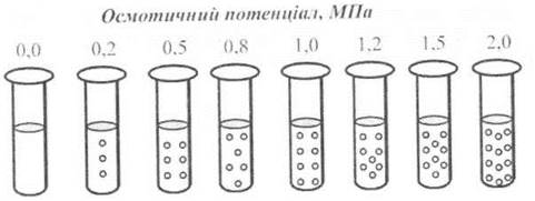
Fig. 6.2. Tissue weight change method (explanation in text).

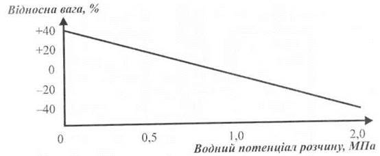
Fig. 6.3. Graph of weight change versus solution water potential.

6.7.2. Thermocouple Psychrometry

A small sample of plant tissue (such as a leaf) is placed inside a chamber equipped with a Temperature sensor—a thermocouple. As water evaporates from the leaf surface, its temperature drops. Because water leaves the plant tissue, the tissue's water potential decreases until a state of equilibrium is reached. When water vapor and plant tissue are in equilibrium, they share the same water potential. Water potential can be evaluated by measuring the water vapor pressure within the chamber, which is temperature-dependent. The temperature measurement relies on two thermocouples forming an electrical circuit. The junction of one thermocouple is located inside the chamber, while the reference junction is maintained at a known constant temperature. If the two thermocouple junctions are at different temperatures, an electromotance (electromotive force) is generated, and an electric current begins to flow through the circuit. This thermoelectric phenomenon is known as the Seebeck effect.

The thermocouple psychrometry method involves using a thermocouple equipped with a silver ring that holds a droplet of water (Fig. 6.4). Initially, water evaporates from the surfaces of both the leaf and the water droplet. Because the chamber is small, the internal atmosphere rapidly reaches saturation. If the plant tissue and the water droplet have equal water potentials, the net water flux from the droplet ceases, and the droplet temperature equals the ambient temperature. However, if the water potential of the plant tissue is more negative than that of the water droplet, water diffuses from the atmosphere into the tissue. The evaporation from the droplet surface—which compensates for the water vapor absorbed by the tissue—causes the droplet-bearing thermocouple to cool down. The rate of mass transfer via diffusion is proportional to the difference in water potential between the droplet and the tissue. Therefore, measuring the cooling rate of the thermocouple allows one to estimate the water vapor pressure in the chamber and the water potential of the tissue. A drawback of this method is the high diffusional resistance to water transport offered by the plant tissue, which introduces measurement errors.

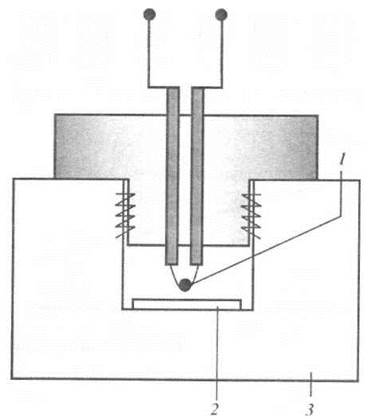
Fig. 6.4. Principle of the thermocouple psychrometry method: 1 - thermocouple; 2 - sample; 3 — thermostat.

A Modification of the thermocouple psychrometry method—known as the isopiestic technique—differs in that a droplet of a solution of known concentration (and thus known water potential) is placed on the thermocouple junction instead of pure water [Boyer and Rnipling, 1965]. If the water potential of the solution exceeds that of the plant tissue, water will move from the solution to the tissue, causing the thermocouple to cool. Conversely, if the water potential of the solution is lower than that of the tissue, the reverse water transport occurs from the tissue to the solution. This process is accompanied by water Condensation on the thermocouple, leading to a rise in its temperature. Obviously, when the water potentials of the solution and the tissue are equal, the water vapor pressures near the thermocouple and the tissue balance out, and evaporative cooling of the thermocouple stops. In this case, the thermocouple temperature reaches ambient temperature. In practice, two solutions of known concentration are used, and the thermocouple outputs are measured for each solution. Since the relationship between the water potential and the thermocouple output signal is linear, a straight line can be drawn between the two obtained points. Extrapolating this line to the point where the output signal equals zero yields the isopiestic point, which indicates zero net water vapor movement between the solution and the thermocouple, corresponding to the water potential of the tissue. This method is characterized by high sensitivity, allowing water potentials to be measured with a resolution of about 0.01 MPa. Limitations of the method include The Need for extremely precise temperature control: a temperature variation of 0.01 °C results in a corresponding water potential error of 0.1 MPa. Consequently, this technique is restricted to laboratory settings rather than field use.

6.7.3. Pressure Chamber

This simple and rapid method is based on measuring the negative hydrostatic pressure in the xylem [Scholander et al., 1965]. It is assumed that the xylem water potential is approximately equal to the average water potential of the entire plant. This assumption is valid because the osmotic potential of the xylem sap is negligible, making negative hydrostatic pressure the primary component of xylem water potential; furthermore, the xylem is in close contact with most plant Cells. To perform the measurement, a leaf or SHOOT is excised from the plant and sealed in a pressure chamber (Fig. 6.5). As a result of xylem tension, sap recedes from the cut surface. To force the water back to the cut surface, pneumatic pressure from a compressed gas cylinder is applied inside the chamber until sap reappears at the cut. This balancing pressure is equal in magnitude (but opposite in sign) to the negative hydrostatic pressure pre-existing in the xylem of the sample prior to excision.

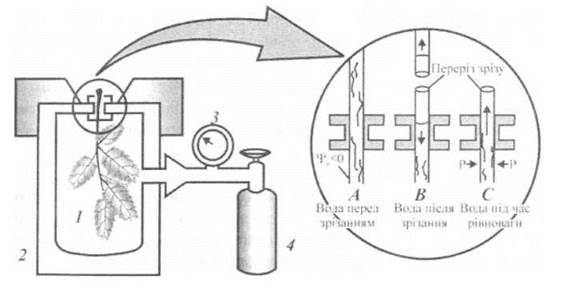
Fig. 6.5. Securing a leaf or shoot in the pressure chamber: 1 - sample, 2 - pressure chamber, 3 - pressure gauge, 4 - gas cylinder.

6.7.4. Nuclear Magnetic Resonance Method

Most water potential measurement techniques require the destruction of samples, making it extremely difficult to monitor dynamic water transport processes in Tissues over time. These drawbacks are absent in nuclear magnetic resonance (NMR) techniques, which are based on the selective absorption of electromagnetic energy by matter, driven by quantum transitions of atomic nuclei between energy states with different nuclear spin orientations.

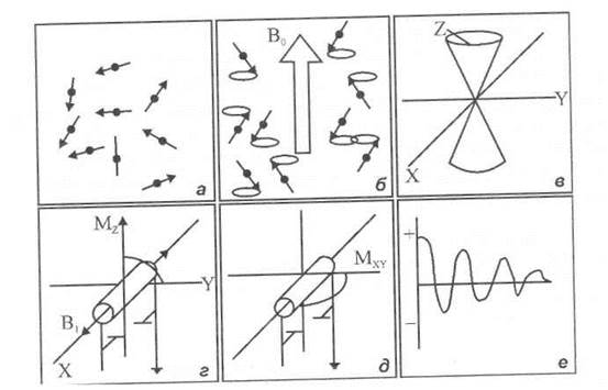
Fig. 6.6. Behavior of nuclear dipole moments in an external magnetic field: a - nuclear dipole moments; b - precession of dipoles around the direction of the external static magnetic field; c - precession of two spins in opposite directions; d - emergence of a net magnetization due to the orientational difference between two groups of dipoles; e - Rotation of the M_z vector by 90° upon applying a π/2 radiofrequency magnetic field pulse; f - waveform of the recorded free induction decay (FID) signal.

It is known that the nuclei of all elements carry a positive electrical charge equal in magnitude to the sum of the charges of the atomic electrons. Due to its intrinsic angular momentum (spin), a rotating Nucleus acts as an elementary magnet. Consequently, The Nucleus is characterized by a magnetic moment whose magnitude depends on The Nature of the nucleus. Nuclei with an even number of protons and an even number of neutrons possess neither spin nor a magnetic moment, whereas nuclei with an even number of protons and an odd number of neutrons have both a spin and a dipole magnetic moment. The magnetic moment is characterized by both magnitude and direction (Fig. 6.6, a). If a sample is placed in an intense, uniform magnetic field B₉, all the dipoles begin to precess around the direction of the magnetic field (Fig. 6.6, b) at the Larmor frequency, which is determined as follows:

where γ is the gyromagnetic ratio.

Furthermore, one group of dipoles exhibits a net orientation along the magnetic field, while the other is oriented against the field (Fig. 6.6, c). It should be noted that in The equilibrium state, the number of dipoles oriented along the field exceeds the number of oppositely oriented dipoles. This can be explained by the fact that in the ground energy state—when the magnetic dipoles are oriented in the direction of the magnetic field—the nuclear energy is lower than in the excited state, which is characterized by an orientation opposite to the magnetic field.

Example. The nuclear magnetic moment behaves like a mechanical system—a gyroscope. When a gyroscope rotates about its own axis, the application of an external force F in the X direction causes the axis of the gyroscope to rotate around this axis rather than around the y-axis, as might seem at first glance. As a result of the external force, the gyroscope will undergo precession in a gravitational field (Fig. 6.7).

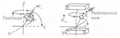
Fig. 6.7. Precession of a gyroscope in a gravitational field.

The energy difference ΔЕ between the levels is proportional to the magnetic induction:

where h is Planck's constant.

The population difference between the ground and excited levels is determined by the expression:

where N_зб and N₀ are the populations of the excited and ground levels, respectively, and T is the temperature.

Example. Determine the Larmor frequency of a proton in a magnetic field, the energy difference between the excited and ground levels, and the relative population difference, given that the magnetic Induction of the external field is B₀ = 2 T, the gyromagnetic ratio of the proton is γ = 42.6 MHz/T, and the temperature is T = 300 K.

Solution. The Larmor frequency can be determined using expression (6.14).

The energy difference between the excited and ground levels is determined using expression (6.15).

The relative population difference is determined as follows:

Due to this difference in magnetic dipoles, a net magnetization M_z is produced, which is parallel to the z-axis of the constant magnetic field.

If an external radio-frequency magnetic field B₁, directed perpendicular to B₀ (Fig. 6.6, d), is applied to the sample via electric current coils, it will interact with the nuclear magnetic moment μ. This interaction becomes pronounced when the frequency ω of the radio-frequency field is close to the Larmor frequency ω₀. If the radio-frequency magnetic field is turned on for a finite time interval t, the magnetization vector M_z will rotate around B₁ by an angle θ = γB₁t. The duration of the radio-frequency magnetic field can be adjusted (a π/2-pulse) such that the vector M_z rotates by 90° (Fig. 6.6, e). After the radio-frequency magnetic field B₁ is switched off, the magnetization vector M_xy undergoes precession around the z-axis at a frequency equal to the difference between the precession frequencies of the two populations of magnetic dipoles—those oriented along the field and those oriented opposite to it. The precession of the magnetization vector M_xy is detected via the electric current induced in the induction coils, whose axis is perpendicular to the direction of the external magnetic field B₀. The recorded signal takes the form of a decaying cosine wave (Fig. 6.6, f).

The magnitudes of the magnetization vectors M_z and M_xy change with time after the radio-frequency pulse is turned off (Fig. 6.8): M_z increases exponentially over time According to the expression:

whereas M_xy decays exponentially:

where T₁ is the longitudinal (spin-lattice) relaxation time and T₂ is the transverse (spin-spin) relaxation time, both of which are crucial diagnostic parameters for assessing sample properties.

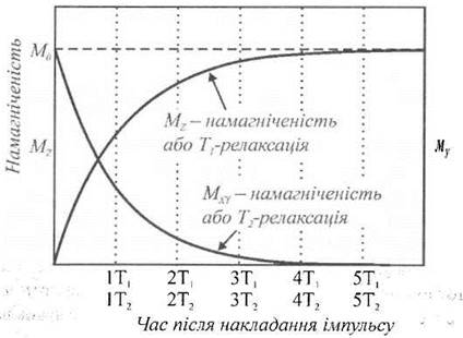
Fig. 6.8. Plot of M_z and M_xy magnetization vector components over time following the radiofrequency pulse cutoff.

The longitudinal relaxation time T₁ characterizes the Influence of the lattice—the nuclear environment formed by the rest of the molecule and solvent molecules. The transverse relaxation time T₂ describes energy exchange processes between neighboring nuclear moments without energy transfer to the lattice. To measure T₁, a π/2 radiofrequency magnetic field pulse is applied, whereas for T₂ measurements, a π pulse is typically used, which rotates the vector M by 180° along the -z direction. The scheme of an NMR spectrometer is shown in Fig. 6.9. It consists of static and radiofrequency magnetic field sources, an induction coil, measuring instruments, and the sample.

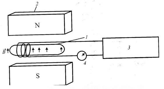
Fig. 6.9. Schematic diagram of an NMR spectrometer: 1 - sample, 2 - magnet, 3 - generator, 4 - detector.

Water activity in a plant is determined by how rapidly water molecules participate in Chemical Reactions or how easily they diffuse to the sites where these reactions occur. The application of NMR techniques makes it possible to evaluate water mobility in complex systems. Fast water molecules are characterized by long equilibrium times, or high values of the relaxation times T₁ or T₂. Conversely, adding a solute to water decreases the relaxation time (Fig. 6.10). In biological macromolecules, the transverse relaxation time T₂ depends on potential conformational changes of water molecules, water-membrane interactions, and the effects of Hydration on Proteins. Therefore, the transverse relaxation time of protons in cells can serve as an indicator of cellular water interactions with membranes or macromolecules. Measuring this parameter is an effective non-destructive method for assessing the physiological state of water within cells.

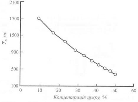
Fig. 6.10. Graph showing the decrease in relaxation time upon The addition of a solute to water.

6.7.5. Measurement of Osmotic Potential

Cryoscopic osmometry involves estimating the osmotic potential of a solution based on its freezing point. A fundamental property of solutions is that their freezing point depends on the concentration of the dissolved substance. For example, a 1 mol·kg^-1 solution freezes at -1.86 °C, whereas pure water freezes at 0 °C. The measurement procedure is based on Cell/15.html">Microscopy of tiny samples—solutions with a volume of 1 nl (10^-9 L)—placed in oil on a Microscope stage maintained at a constant temperature (Fig. 6.11). Initially, plant sap exuded from cells is observed; due to the small Sample size, thermal equilibrium is reached almost instantly. The sample temperature is then lowered to -30 °C to freeze it. Afterward, the temperature is slowly raised while monitoring the melting process under a microscope to record the temperature at which the last ice crystals melt (recall that the freezing and melting points are identical). The osmotic potential is estimated as Ψ = RTC_c, where R is the universal gas constant, T is the absolute temperature, and C_c is the solution concentration. This technique allows measurements to be performed on droplets extracted from single cells.

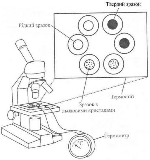
Fig. 6.11. Cryoscopic osmometry.

6.7.6. Measurement of Pressure Potential

The pressure probe is a micromanometer designed to measure turgor pressure in plant cells [Green and Stanton, 1967]. A Glass capillary with a diameter of 2-7 µm, connected to a pressure chamber, is filled with silicone oil—an incompressible liquid that is easily distinguished from water under a microscope. The probe is equipped with a micro-plunger to adjust the pressure. When the tip of the capillary is inserted into a cell (Fig. 6.12), cell sap enters the capillary due to turgor pressure. The researcher then turns the probe's plunger knob to reposition the boundary between the two phases (sap and oil) back to the tip of the capillary. At this point, the original cell volume is restored, and the internal cell pressure is precisely counterbalanced by the pressure generated in the capillary by the micromanometer. This pressure, measured by an electronic pressure transducer, corresponds to the turgor pressure. The method causes minimal disruption and makes it possible to study small cells (down to 20 µm in diameter) containing only a few picoliters (10^-12 L) of fluid.

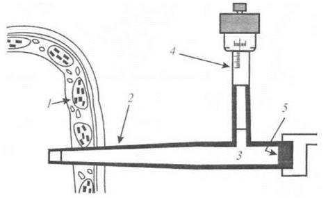
Fig. 6.12. "Pressure probe"—a micromanometer for measuring turgor pressure in plant cells [Green and Stanton, 1967]: 1 - cell, 2 - microcapillary, 3 - oil, 4 - micrometer, 5 - pressure transducer.

6.7.7. Pressure-Volume Curve Analysis

One of the best graphical Methods for measuring water potential is based on the construction and analysis of pressure-volume curves. These curves characterize the relationship between water content in plant tissue and the COMPONENTS OF WATER potential. The osmotic potential Ψ of the tissue is related to its water deficit as follows:

where Δ_в is the water deficit, φ is the osmotic coefficient, ρ is the density of water, R is the universal gas constant, T is the absolute temperature, and N is the total number of moles of solute in the sample.

Using the latter equation, the pressure-volume relationship can be expressed as:

where p is the pressure corresponding to the equilibrium state in the pressure chamber, V₀ is the initial water volume, V_в is the total volume of water expressed, and Ψ_m is the turgor potential of the tissue.

If a certain amount of water is removed from a shoot, the turgor potential becomes zero, and the above equation takes the following form:

This equation describes the linear dependence of 1/Ψ_s on the water deficit caused solely by the osmotic potential.

The measurement procedure involves cutting a shoot or leaf, weighing the sample, and placing it in a saturation chamber. After complete rehydration, the sample is weighed again and placed in a pressure chamber with a moist lining. The humidity in the chamber is set high enough to prevent evaporation from the sample surface. The pressure in the chamber is gradually increased in discrete steps (by increments of about 6 atm), and the volume of expelled water is measured at each step. After each pressure increase and volume measurement, equilibrium is re-established in the pressure chamber. To do this, the pressure is slightly decreased before the next step, equilibrium is allowed to set in, and a new value of the sample's water potential is determined. After 10–15 such measurements, the sample is removed from the chamber, weighed, dried, and weighed again. Next, a plot of (1/Ψ_в) = f(Δ_c) is constructed, where Ψ_в is the water potential. The final points of this curve are approximated by a straight line that intercepts the ordinate axis at point A, which corresponds to the osmotic potential at full turgor 1/Ψ_s¹⁰⁰, and the abscissa axis at point D, which makes it possible to determine the relative water content in the apoplast. The curvilinear section of the curve allows for the Assessment of the influence of the turgor potential Ψ_m on the total water potential Ψ_в (Fig. 6.13). The point where METABOLISM/18.html">The Influence of the turgor potential is absent corresponds to the osmotic potential Ψ_s⁰ at the loss of turgor potential (point B) and the magnitude of the water deficit at the loss of turgor potential (point Q). The difference between the curvilinear and rectilinear sections of the curve characterizes the volumetric modulus of elasticity E. A steeper curvilinear section corresponds to higher values of the modulus of elasticity. It should be noted that the modulus of elasticity decreases with increasing water deficit and decreasing turgor potential.

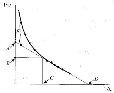
Fig. 6.13. Graphical method for measuring water potential based on the construction and analysis of pressure-volume curves to evaluate the relationship between water content in plant tissue and water potential components (explanation in the text).