Fundamentals of Bioinformatics - Ogurtsov A.N. 2013

Information Principles in Biotechnology
Protein Analysis and Prediction
Prediction of Protein Secondary Structure

One of the most critical tasks in sequence analysis is the accurate prediction of $\alpha$-helix, $\beta$-strand, and other Secondary Structure elements within a protein amino acid chain.

Structure prediction from an Amino Acid Sequence begins by analyzing a database of known structures. Searching these Databases aims to uncover all potential correlations between a protein's sequence and its structure.

The quality of secondary structure prediction depends on how accurately the types of secondary structure elements are recognized in known folds, as well as on the precise Determination of the Location and length of these elements. The MAIN TYPES OF secondary structures examined for sequence Variability include $\alpha$-helices, $\beta$-structures, and Supersecondary structures (see [9], sec. 4.2).

Currently, the most widely used Protein secondary structure prediction Methods are:

1) the Chou-Fasman methods (P.Y. Chou, G.D. Fasman (1974)) and the Garnier-Osguthorpe-Robson (GOR) method (J. Garnier, D.J. Osguthorpe, B. Robson (1978));

2) artificial neural network modeling methods;

3) nearest-neighbor search methods.

The Chou-Fasman method, introduced by Peter Y. Chou and Gerald D. Fasman, is based on the assumption that each amino acid individually influences the secondary structure within a specific sequence window. It relies on analyzing the occurrence frequencies of each of the 20 Amino Acids in $\alpha$-helices, $\beta$-strands, and $\beta$-turns. Furthermore, the algorithm built upon this approach utilizes a special set of secondary structure prediction rules. Initially, the algorithm scans the sequence to find a short subsequence of amino acids showing a high propensity for forming a nucleation site of a specific structure type.

Prediction of $\alpha$-helices is considered reasonably reliable if four out of six Amino acids have a high probability (>1.0) of being in an $\alpha$-helix. As for predicting $\beta$-strand nucleation propensity, it is deemed correct if for every Five amino acids in the sequence, three have a $\beta$-strand probability of >1.0. The algorithm then extends the nucleation regions in both directions until the probability values for a group of four amino acids drop below 1.

If both $\alpha$-helical and $\beta$-structural regions can be predicted for a given sequence segment, the prediction with the higher probability is accepted.

The prediction of $\beta$-turns (Figure 81), which enable the peptide chain to reverse direction by approximately 180 degrees over a segment of 4 amino acid residues (residues 1 and 4 being hydrogen-bonded), is based on a somewhat different principle.

Class="center">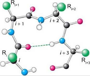

Figure 81 - Scheme of a $\beta$-turn

The algorithm models turns as tetrapeptides and calculates two probabilities.

First, similarly to $\alpha$-helix and $\beta$-strand predictions, the algorithm computes the average probability of turn formation for each of the four amino acids.

Second, it determines the probabilities of specific amino acid combinations appearing in a turn starting from a given tetrapeptide position.

Then, the algorithm multiplies these four probabilities calculated for the group of four amino acids in the modeled sequence, yielding the probability that the given tetrapeptide forms a turn.

A turn prediction is considered correct if the first probability value exceeds the probability of an $\alpha$-helix or $\beta$-strand occurring in that region, and if the second probability value is greater than $7.5\cdot 10^{-5}$.

The GOR method rests on the assumption that amino acids adjacent to a central amino acid residue also influence the secondary structure that the central residue is likely to adopt. This method relies on information theory principles when making predictions. The GOR algorithm scans known secondary structures and determines the frequency of specific amino acids in each structure type. Additionally, it determines the frequencies of all 20 amino acids across eight neighboring positions (extending from the N- and C-termini of the central amino acid), resulting in a total of 17 examined positions, including the central one.

Prediction using neural networks. Neural networks are a class of general computational architectures that model the anatomy and physiology of biological neural systems. They have been successfully applied to a broad range of pattern recognition, Classification, and decision-making tasks.

In a computational schema, a single "neuron" is a graph vertex with one or more incoming edges (inputs) and one outgoing edge (Figure 82(a)).

Figure 82 - Neural networks: a - graph vertex; b - simple neural network diagram

Using a physiological metaphor, a neuron fires a signal if its output is 1, and does not fire if its output is 0. Model Neurons may vary in their number of inputs and outputs, as well as in the mathematical function used to calculate their output (Figure 82(b)).

To form a network, multiple neurons must be created and the outputs of some neurons connected to the inputs of others. Some vertices provide inputs for the entire network (the input layer), while others have outputs directed outward (the output layer). Additionally, there are neurons that are not directly connected to the outside world (the hidden layer) (Figure 82(b)).

Unlimited complexity is achievable by creating and connecting neurons and defining strictness of connections; that is, instead of simply summing input signals i₁ + i₂ + i₃, one can use weighted input sums, such as 9i₁ + 5i₂ + i₃, making the network more sensitive to input number 1 and less sensitive to input number 3. Biologically, this corresponds to altering synaptic strength. (Synaptic strength is the magnitude of change in the transmembrane potential resulting from the activation of postsynaptic receptors by Neurotransmitters).

The property of a neural network that determines its computational power lies in the fact that weights can be treated as variables and computed during the training process for specific cases. To train a neural network, it is applied to various Examples and its output is compared against the correct solution. If the output does not match, the parameters are adjusted accordingly. During training, the network topology remains unchanged; however, if the weight of a particular connection becomes 0, it is equivalent to severing that connection.

The type of neural network that can be applied to protein secondary structure prediction is shown in Figure 83.

The input layer (IL) scans the sequence using a 15-residue sliding window, meaning a sequence fragment of 15 elements is analyzed at a time. The prediction corresponds to the central residue (at the top, indicated by an arrow). The window is then shifted one position to the right along the sequence, and the next prediction is made. Each of the 15 positions (amino acids) in the window corresponds to 20 neurons, one of which is active (black circle).

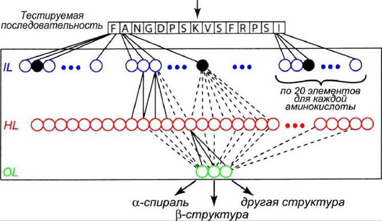
Figure 83 - Neural network for protein secondary structure prediction

The hidden layer (HL) contains 15x20=300 neurons connected to both the input and output. Every neuron in the hidden layer is connected to every neuron in the input and output layers (not all connections are shown in the figure).

The output layer (OL) consists of only three neurons that simply record the prediction: an alpha-helix, a beta-structure, or neither.

Evolutionary information is a crucial type of data that can be utilized in secondary structure prediction. Multiple Sequence Alignment contains significantly more information than a single sequence. The conservation of secondary structure in homologous Proteins indicates a strong sequence-structure relationship, which allows for higher profile weights and more robust predictions. Most neural network-based secondary structure prediction methods incorporate not only positional conservation scores but also profile weights in their input layer.

Furthermore, utilizing two tandem (consecutive) neural networks allows for accounting for the conformational correlation of neighboring residues. Predictions of the states of several consecutive residues made by a network similar to the one shown in Figure 83 are combined using another network that generates the final result.

In the neural network approach, computer programs are trained to recognize regular amino acid combinations found in known secondary structures and to distinguish these combinations from other amino acid groups not residing in such structures. Such neural network models extract the majority of their sequence information through algorithmic interpretation.

Notable neural network simulation programs include:

- PHD (http://www.predictprotein.org/);

- NNPREDICT (http://www.cmpharm.ucsf.edu/~nomi/nnpredict.html).

Nearest-neighbor prediction. Much like neural network methods, nearest-neighbor approaches are based on machine learning principles. They predict an amino acid's propensity within a query sequence to adopt a specific secondary structure conformation. To achieve this, the algorithm compares the query sequence with similar sequences of known structure.

The algorithm moves a variable-length window across a set of 100–400 training sequences with known structures, compiling a large list of short sequence fragments as test candidates.

Next, the minimum mutual sequence similarity is recorded, along with the secondary structure corresponding to the central amino acid in each window. The algorithm then selects a window of the same size from the query sequence, compares it against each of the aforementioned candidate fragments, and identifies the 50 fragments yielding the best matches. Finally, based on the frequencies of occurrence of the known Introduction/11.html">Secondary structure of the central amino acid across each of these 50 fragments, a secondary structure prediction is generated for the central amino acid in the query sequence window.

Secondary structure propensity. Over time, numerous attempts have been made to predict secondary structure directly from The amino acid sequence. Observations on model polypeptide solutions have demonstrated that amino acids exhibit high variability in their propensity to form regular Conformations.

The earliest attempts at secondary structure prediction were based on the parameterization of physical models. For instance, physicochemical studies of model Polypeptides established that an amino acid's propensity to propagate helices can differ from its propensity to initiate them.

As mentioned above, Chou and Fasman proposed an approach based on a statistical model. According to this method, the frequency of a specific amino acid occurring in a given conformation is compared against the average frequency of all known amino acids (from the alphabet) occurring in that same conformation. The resulting ratio expresses that amino acid's propensity to appear in the given conformation. Based on these values, amino acids were classified into distinct categories, which subsequently served as the foundation for formulating secondary structure prediction rules.

The Chou-Fasman and GOR methods rely on METABOLISM/2.html">THE CONCEPT OF amino acid propensities for forming specific secondary structures. As it turns out, amino acids show preferences for certain secondary structure states, as reflected in Table 20.

A probability value of 1.0 indicates that an amino acid's propensity for the corresponding secondary structure equals the average propensity of all known amino acids; values greater than 1.0 indicate above-average propensity, while values less than 1.0 indicate below-average propensity.

Table 20 - Amino acid propensities for forming alpha-helices and beta-structures

The values were calculated by dividing the frequency of a given residue in a specific secondary structure by the average frequency of all known residues in that secondary structure. For example, glutamic acid shows a clear preference for a helical secondary structure (1.59 vs 0.52), whereas glycine exhibits a below-average propensity (0.43 and 0.58) for both types of regular secondary structure, indicating its preference for loops.

However, the accuracy of these early methods, which relied on the local Amino Acid Composition of individual sequences, was rather low, allowing the correct secondary structure state to be predicted for no more than 60% of the residues.

The intrinsic propensity of amino acids to form ß-turns. The frequency of amino acid pairs occurring in ß-turns was calculated by analyzing data from protein crystal structure studies. The following frequencies were noted: Pro-Asn (63%), Pro-Phe (50%), Pro-Gly (38%), Pro-Ser (31%), and Pro-Val (8%). However, a statistical analysis based on a different criterion for assessing ß-turn propensity revealed a significant difference in the order of preference. For instance, an investigation of a set of protein structures from the database established the following order of preference: Pro-Gly > Pro-Asn > Pro-Ser > Pro-Val > Pro-Phe.

The propensity for ß-turn formation was evaluated by measuring the standard Gibbs Free energy of peptide cyclization in model Cys-Pro-X-Pro tetrapeptides. The following order of preference was observed: Pro-Asn > Pro-Gly > Pro-Ser > Pro-Phe > Pro-Val.

NMR measurements of the Temperature dependence of chemical shifts in model Peptides such as Tyr-Pro-X-Asp-Val enabled the identification of ß-turn families. According to the NMR spectroscopy data, the ß-turn families follow the order Pro-Gly > Pro-Asn > Pro-Phe > Pro-Ser > Pro-Val.

A joint analysis of thermodynamic, NMR, and crystal structure (statistical) data indicates that the order of preference is as follows: Pro-Gly, Pro-Asn > Pro-Ser > Pro-Val.

Although the relative position of the Pro-Phe pair appears highly variable in this series, other peptides exhibit a clear correlation between the statistical preferences calculated from database protein structures and those derived from thermodynamic analysis and NMR spectroscopy of model compounds.

Rotamer libraries. A rotamer is defined as one of a set of conformers resulting from restricted rotation around a single chemical bond.

A conformer, or rotational isomer, is a specific folded state or structure of a protein characterized by low energy, meaning it is thermodynamically stable under physiological conditions.

Investigations into the conformational preferences of side chains have demonstrated that certain side-chain conformational variants have a significantly higher probability of occurrence than others. These findings motivated researchers to conduct a series of studies aimed at determining the probability function for a given amino acid's side chain to adopt a specific conformation, as well as establishing the dependence of side-chain conformation on the backbone conformation.

Thanks to the substantially expanded volume of databases, numerous rotamer libraries have been developed. Rotamer libraries can be utilized in molecular modeling: an algorithm extracts the most probable side-chain conformations from them and adds them to the backbone of the macromolecule.