BOTANY VOLUME 4 - ECOLOGY - 2007

14. ECOLOGY OF POPULATIONS AND PLANT COMMUNITIES

14.3. Plant Ecology

When analyzing individual, locally circumscribed plant groupings, one repeatedly discovers the co-occurrence of characteristic taxa.

In most cases, this is not a random proximity, but rather a very specific Selection of species from the total local flora, driven by environmental factors (see Fig. 14.1). Furthermore, the Qualitative and quantitative COMPOSITION OF THE community often reflects the prevailing environmental conditions with surprising precision.

Plant communities are combinations of populations of various species that depend on the abiotic environment and biotic interactions. Their formation follows a regular sequence (succession) from pioneer groupings to mature "climax" communities; when these are disrupted (either entirely or patchily), development resumes from a characteristic intermediate stage toward the climax typical of those conditions (see Fig. 14.14). Disturbances (such as hurricanes, fires, flooding, or animal trampling) can deflect succession in a different direction or halt it at an intermediate stage for a long time. Although the biosphere Functions as an integrated whole, adjacent plant communities are usually well-differentiated from one another, separated by boundaries or transition zones (gradual transitions are ecotones, sharp transitions are ecoclines; these English terms are commonly used). Examples include the transition from forest to grassland, or from wetland to dryland vegetation. The reasons for a species' success (presence) or failure (absence) lie in its ability to reproduce successfully under specific local conditions, with the critical phase for survival potentially corresponding to any stage of The life cycle—from seedling establishment to the successful production of diaspores. This falls within the realm of population ecology (see 14.1.3). The Subject Matter of plant ecology is the spatial and temporal Structure of Plant communities and the identification of functionally significant types and their relationships. It also involves formulating hypotheses to explain the structure

of interaction networks—both interspecific and intraspecific—from a process-oriented perspective (see Chapter 13). One of the key tasks of ecology is simply the Water/301.html">Description and Mapping of vegetation.

Depending on the objectives, geographic area, and scale, as well as spatial and temporal approaches, there are numerous ways to define Abstract vegetation types of various ranks based on field descriptions:

✵ by species composition (Taxonomy) — plant communities;

✵ by dominant physiognomy (morphotypes) — plant formations;

✵ by spatial relationships (habitat similarity / spatial arrangement) — vegetation complexes;

✵ by temporal sequence (developmental stage) — successional series.

14.3.1. Structure of Plant Communities

A preliminary systematic categorization of the plant cover already allows us to appreciate the wide variety of approaches available for analyzing the underlying patterns and relationships. In a mixed beech forest, one is immediately struck by the population STRUCTURE OF THE dominant beech trees, which comprises a mosaic of seedlings, saplings, dominant older trees, and finally dying trees (uprooted by wind or damaged by parasitic Fungi), felled logs, and decomposing fallen trunks. The understory, subordinate and distributed patchily in response to microtopographic and soil variations or light availability, consists of herbaceous plants, graminoids, mosses, and Lichens (Fig. 14.27). Spring-flowering geophytes, such as Anemone nemorosa, completely disappear above ground in summer and autumn, making way for the fruiting bodies of macrofungi that live in mycorrhizal Symbiosis with the beech or, alongside Bacteria and small invertebrates, participate in the decomposition of leaf litter. Other subordinate elements of the biocoenosis are found at the base of tree trunks (bryophytes) and on their bark (aerophytic Algae and crustose lichens).

Class="center">Fig. 14.27. Biocoenotic components (synusiae) in a Central European mixed beech forest in late summer: A — leaf-litter-filled depressions with relatively moist, neutral humus soils (containing bacteria, fungi, and small invertebrates), bordered by indicators of moisture and soil nutrient status: a — bugle (Ajuga reptans), b — wood violet (Viola reichenbachiana); B — micro-elevations free of leaf litter, featuring drier, slightly acidic brown forest soils with a terrestrial moss and lichen synusia: c — cypress-leaved plait-moss (Hypnum cupressiforme), d — white moss (Leucobryum glaucum), e — cup lichen (Cladonia pyxidata), f — micro-elevations with fruiting bodies of the woolly milkcap (Lactarius vellereus; forming mycorrhizae with Fagus) and rosette-forming herbaceous plants (hemicryptophytes) indicative of acidic, nutrient-poor soils, g — white wood-rush (Luzula luzuloides), h — wall hawkweed (Hieracium murorum), i — wavy Hair-grass (Deschampsia flexuosa); C — trunk base with various mosses (Hypnum, Plagiothecium); D — beech bark with a synusia of epiphytic algae (Pleurococcus) and crustose lichens (such as Graphis scripta); E — decaying tree stump colonized by fungi (fruiting bodies of the turkey tail, Coriolus versicolor)

Such comprehensive inventories can only be conducted through multifaceted (and often highly labor-intensive) research. Within a carefully selected sample plot, it is first necessary to record the species composition and life-form spectrum of the plant community, as well as to analyze its vertical stratification, the alternation of large- and small-scale biotopes, and its developmental periodicity. Such general descriptions of the vegetation and its condition subsequently serve as the foundation for defining and describing plant communities.

In German, the term "Struktur" refers to any form of spatial and hierarchical subordination or system of relationships. When English-language specialized literature refers to "community structure" or "canopy structure," it usually implies geometric structure in the sense of "architecture." The German designation for the species composition of a plant community—Struktur des Bestandes (stand structure = taxonomic structure)—corresponds to the English equivalent "community composition."

The starting point for vegetation analysis is the inventorying of small sample plots. The selection and size of such plots depend on which biocoenosis (or part thereof) is to be characterized. To account for all characteristic trees of a Central European forest, a minimal area of about 500 m² is required, whereas species-rich tropical rain forests may necessitate an area of roughly 1 ha. Conversely, for the description of grasslands and turf communities, 10–100 m² is usually sufficient, and for moss and lichen communities, merely 0.1–4 m². In alpine meadows on granitic schists in northern Scandinavia, an area of about 1 m² may harbor up to 50 species of angiosperms. Expanding the area to 100 m² may increase the species count to 60, and to 1 km², up to 80. Thus, a 1 m² plot already captures two-thirds of the regional species list. Having data on the species-area relationship enhances the value of biodiversity assessments (e.g., species counts). The species-area curve (Fig. 14.28) makes it possible to determine the plot size (minimal area) required to obtain a reliable sample containing over 95% of the total species list. Different plot sizes can be achieved either by successively expanding a starting plot or by adding other plots distributed randomly across the total area

area. The two approaches are not entirely equivalent; generally, the second method is more objective and preferable.

Fig. 14.28. Minimal area, or the smallest plot size that contains the complete species Complement of a plant community (> 95% of all species). This can be determined by successively doubling sample plots (A — single-plot method) or by accumulating additional data from plots of the same size (B — multi-plot method). The result is expressed as a species accumulation curve (C), which shows the plot size or number of replicate plots beyond which no significant (> 5%) increase in species richness is to be expected. Typical minimal areas for a single plot in nutrient-poor grassland or alpine meadow are 10–25 m²; in the forest herbaceous layer, 100–200 m²; in relatively undisturbed temperate forest, 500–1,000 m²; and in tropical rain forest, more than 1 ha. The shape of the species-area curve provides insight into the homogeneity of the plant community

For the Classification of plant communities to define community types (formerly known as phytosociology), a range of parameters is used, which can be divided into two main groups. One group describes the growth patterns of individual species within a sample plot, which must at least equal the size of the minimal area. The other group encompasses metrics derived from comparing A large number of such plots.

Within a sample plot, one can determine or measure: population density, or Abundance (number of individuals per unit area), cover (the percentage of ground covered by the vertical projection of a species' individuals, often referred to as spatial dominance), and frequency (the percentage of subplots within the sample plot in which a species occurs). A high frequency of the more important (abundant) species indicates high homogeneity of the plant community (whereas the reverse indicates heterogeneity).

Qualitative attributes include sociability (growth in groups or solitarily) and dispersion (regular or irregular spatial arrangement, a trait closely related to frequency; Fig. 14.29). The vigor index can also be used as a measure of a species' performance, taking its productivity into account.

Fig. 14.29. Examples of species distribution within a plant community, reflected in varying frequencies across a sample plot:

A — regular distribution (found by chance in arid regions to "maintain distance", as well as in monoclonal and anthropogenic communities); B — random distribution (e.g., in unstructured ruderal patches, otherwise rather rare); C — grouped or clumped distribution (frequently found in natural grasslands and primary forests); D — patchy distribution, restricted to discrete spots (patches), often associated with localized disturbances or clones

A comparison of a large number of such descriptions allows us to determine the constancy of a species (the probability of its occurrence as repeated appearances across different sample plots, analogous to the frequency index within a sample plot). The degree of affinity of individual species for particular communities is referred to as their fidelity. Furthermore, species with very high fidelity (and typically higher abundance) are characteristic and are termed character species or characteristic species; others, quite typical and also faithful, yet less strictly bound to this association, are designated as companion species, while the remaining ones are classed as accidentals. Species that divide communities of the same rank into subgroups (e.g., subassociations) are called differential species or discriminating species. While not dominants, they exhibit a strong and specific affinity (fidelity) to the corresponding subgroup and high constancy within it, but not at the next higher sociological rank. Differential species,

as a rule, serve as good indicators of specific environmental conditions.

Most commonly, species lists (known as relevés) are accompanied by estimates of dominance (cover) or individual density for separate species (dominance and abundance are combined into a single measure of species vigor). This methodological alternative arises from the need to distinguish between species with narrow, vertically oriented leaves and those with broad, horizontally disposed ones. Rosette-forming species may exhibit a relatively low individual density despite high cover. Conversely, some grasses achieve a relatively low cover despite high SHOOT density. For clonal plants or those producing numerous shoots, technical reasons dictate that shoots (ramets) are evaluated rather than genetic individuals (genets). Abundance (= density) values are usually denoted using an approximate rating scale (Table 14.2).

Table 14.2. Evaluative classification of abundance values

This rating scale, based on estimation, is frequently supplemented or modified at the lower end for specialized practical purposes. Essentially, it corresponds to modified cover-estimation indices, whereby dominant species are often rated somewhat lower and rare ones higher. Precise quantitative data can only be obtained by harvesting all vegetation, followed by counting and weighing all individuals. A very reliable quantitative estimate of cover is achieved via the "point-quadrat" method, in which needles are lowered into a dense, coordinate-gridded frame, and the first contact of a needle with an individual of a given species at a grid intersection point is recorded.

Every vegetation description is supplemented with habitat-characterizing data, such as topographic position, altitude, aspect, slope steepness, soil type, parent material, land use, etc. Gradual or abrupt changes in species composition along a specific environmental gradient (e.g., altitude, moisture availability, salinity, pH, light intensity) are best represented in the form of a vegetation transect (see Fig. 13.28). This serves as a starting point for the most objective possible delimitation of plant communities. Often, the approximate value of the characterized attributes lies in the fact that, on the one hand, these features (especially the cover-abundance ratio) allow the presence of a species to be "weighted", while, on the other hand, due to a large number of replicates, occasional relative anomalies do not disrupt the emerging, sufficiently clear overall picture, thereby enabling quantitative comparisons.

Table 14.3. Life-form spectra (% contribution of respective species) of some major formations and ecological series (see Fig. 14.19, 14.42)

Decisive attributes for the overall habit of any plant community are the Morphology (form) of the species, as well as their life forms and growth forms (see 4.2.4). According to W. Rauh, growth form is the organizational principle or structural plan, whereas life form is what can be realized ad hoc in the living space within the latitudinal belt whose conditions permit it. Thus, the growth form of a tree may well be "compressed" into a shrub form under certain environmental conditions. Admittedly, the terminological distinction plays virtually no role in the literature, with both concepts being used synonymously (referred to as life form in German-language literature, and growth form in English). A wide variety of life forms exist across different zones and major vegetation types of the Earth (see Fig. 14.42, Table 14.3), whose contribution to vegetation structure determines its vertical stratification. Only primary pioneer biocenoses, as well as those under extreme conditions, have few layers (strata) or are single-layered. Most natural forests feature:

✵ a tree layer, often with lianas and epiphytes, which may itself be subdivided into multiple strata;

✵ a shrub layer, including young trees;

✵ an herb layer with dwarf shrubs and subshrubs, including tree seedlings;

✵ a moss and lichen (ground) layer.

This above-ground vertical Structuring of vegetation corresponds to the less-studied subterranean ROOT system stratification in the rhizosphere (see Fig. 13.24). Clearly, the differentiated exploitation of the aerial space and the soil profile provides opportunities for better resource utilization (light, moisture, soil nutrients, see 14.2.4 2).

The traditional division of plants into shallow- and deep-rooted is overly simplistic and functionally poorly justified. Nearly all perennial plants possess both surface and deeply penetrating roots, though their ratio varies among species and is heavily dependent on moisture and nutrient availability. A small number of deep roots (which are often inconspicuous) ensure a minimal supply of moisture to the plant even during critical periods (at least to cover the very low cuticular water loss through stomatal apertures), while surface roots secure the uptake of the bulk of nutrients from the biologically highly active upper soil layer. In periodically dry regions, rooting depth is closely correlated with the seasonal rhythm of shoot activity. Species that remain active (green) during the dry season have deeper roots than deciduous ones. In Central European moderately dry grasslands on limestone, over 80% of all roots are located in the upper 20 cm of the soil profile, although individual roots penetrate down to 6 m, as visible on vertical exposures. Maximum root depths exceeding 15 m can be observed as a rule rather than an exception in most periodically arid Regions of the Earth (Table 14.3).

Vegetation cover is also structured horizontally. Depending on the extent of plant-free surface, one distinguishes between open and closed vegetation. Even within a seemingly homogeneous stand, a differentiated horizontal distribution of species can frequently be observed in the form of a distinct pattern, mosaic, or coalition (certain species grouping together or standing far apart, see Fig. 14.29). Minor elevations or depressions in microrelief (see Fig. 12.13) cause variations in moisture and nutrient supply (see 13.6.2) and, consequently,

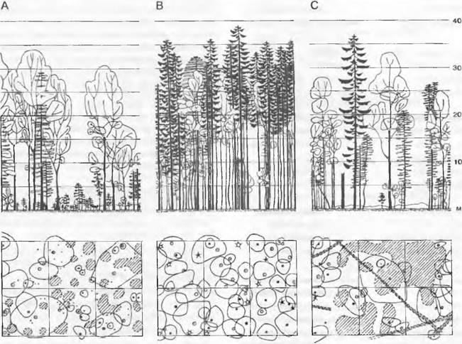
in species abundance. The vegetation cover itself also creates various microhabitats (see Fig. 14.27). Of particular importance are gaps in the canopy, formed through the mortality of individuals, as these create open space for the establishment of new individuals. A prime, typical description of forest development focuses precisely on the dynamics within such gaps (gap dynamics, gap models). It primarily addresses the longevity of these gaps and the succession that unfolds within them. Figure 14.30 illustrates the cycle from regeneration (A) to optimum (B) and breakdown (C) of a forest stand. This cycle depends on the lifespan of the dominant individuals. In so-called windfall gaps, regeneration does not occur immediately, but proceeds through stages of short-lived pioneers, followed by fast-growing, intermediate (seral) species, and finally by young plants of the originally dominant species (see 14.3.2). At the same time, the establishment of young plants can succeed more effectively directly under the protection of other individuals (facilitation — e.g., cacti establish better under the shelter of desert shrubs, a phenomenon well documented in the saguaro cactus — Carnegiea gigantea).

Fig. 14.30. Cyclical regeneration of a mountain spruce-fir-beech primeval forest in the Eastern Alps (Rothwald near Lunz, 1,000 m): A — rejuvenation phase with abundant undergrowth in "gaps" (windthrow sites); B — optimum phase with densely closed canopies and conifer dominance; C — breakdown phase of the overmature community (numerous standing and fallen dead trees, increased beech participation, reappearance of undergrowth). Vertical and horizontal vegetation profiles: • spruce (side branches filled in dark); fir (side branches unfilled); beech (foliage canopies depicted schematically); fallen trunks, undergrowth — hatched

Finally, a strongly ordering/structuring element is also the temporal sequence, or periodicity, in The Development of individual plants and communities as a whole. Phenological phases such as leaf unfolding, flowering, fruiting, and leaf senescence are particularly crucial (Fig. 14.31). Together, they give rise to different "aspects" (visual appearance) of the plant community across various seasons of the year.

Fig. 14.31. Seasonal development (phenology) of character species in a humid oak-beech forest in northwestern Germany. Black indicates the development of current-year leaves, horizontal lines overwintered leaves, and vertical lines flowers

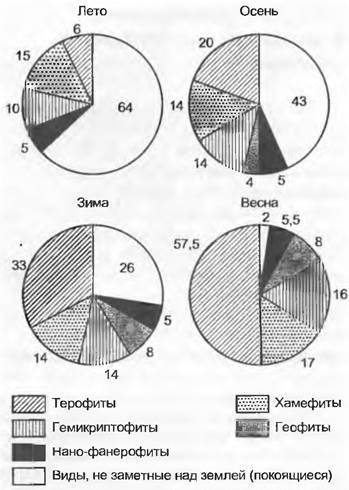
When comparing the seasonal development of species in moist oak-beech forests (see Fig. 14.31), it is notable that the foliage on deciduous trees, which are more exposed to winter frosts, unfolds late. Ilex remains the only evergreen. The period before or during leaf unfolding is more favorable for flowering, particularly for wind-pollinated (anemophilous) trees. This bright period is also utilized by light-demanding geophytes, which complete their development within a short spring window. The remaining herbaceous layer species are shade-tolerant; growing directly near the soil surface (providing frost protection), many retain their leaves throughout the winter. A partial or complete summer dieback of therophytes (annuals) and geophytes (bulbous and tuberous plants, Fig. 14.32) is a particularly characteristic seasonal aspect of Mediterranean vegetation.

Fig. 14.32. Seasonal Changes in the representation of plants from different life forms in the composition of Mediterranean rocky scrub (Brachypodietum ramos near Montpellier, southern France). Percentages are calculated based on the total number of species (111)

Thus, plant communities exhibit an ordered spatio-temporal structure. Their high species richness and diversity of life and growth forms are often spatially, functionally, and seasonally linked to the availability of ecological niches. The relationships between species can range from mutually complementary to dependent, and disturbances positively influence coexistence (see 14.2.4.1).

14.3.2. Formation and Dynamics of Plant Communities

The plant cover is in a state of continuous change (see above) and appears in the same habitats with a set of species, life-form spectrum, and dominants that vary depending on the successional phase. This is clearly evident from long-term analyses and observations on permanent monitoring plots (permanent plots, permanent quadrants; Fig. 14.33). However, comparisons of various patches of established vegetation in similar habitats also provide a clear picture of ongoing succession (Fig. 14.34).

Fig. 14.33. Sequential vegetation change (succession) over 4 years on a permanently monitored plot (1 m²) that was initially unvegetated. Dried peat of a heath bog (Hilden, Rhineland): a — Agrostis sp.; b — Molinia caerulea, c — Sphagnum papillosum, d — S. auriculatum, e — Erica tetralix, f — Juncus bulbosus, g — J. squamosus, h — Dicranella cerviculata-, i — Carex panacea-, j, k — Eriophorum angustifolium, I — Cerastium sp.; m — Polygala serpyllifolia: n — Rhynchospora alba

Fig. 14.34. Secondary forest regrowth on an abandoned field in the temperate zone (North America; Brookhaven, New York). After approximately 8 years, herbaceous plants and graminoids are replaced by summer-green shrubs, which in turn are replaced after 30 years by deciduous forests that stabilize by 150 years into a climax forest dominated by summer-green oaks and pines. During this progressive succession, net primary production (A, o—o) and plant community biomass (B, □—□) increase up to the climax stage; conversely, the number of vascular plant species (C, ▲—▲) declines after peaking in the late herbaceous phase, as does the number of adventive species (D, ∆—∆), which are eliminated during the shrub stage due to competition

The reconstruction of long-term vegetation development is based on fossil remains (pollen) and soil profile properties (fossil soil horizons and "fire" horizons). In semi-arid regions, information regarding historical shifts between dominant C3 and C4 plants can be tracked by analyzing carbon isotope ratios in humus (see 13.7.4). Particularly instructive are experiments where succession can be observed following the exclusion of disturbances (fencing off herbivores, fire suppression).

Initial colonization and subsequent changes in species composition require dispersal elements (see diaspores) brought in from outside or present in a dormant state in the soil seed bank. It has been established that up to 50,000 viable seeds can be present per 1 m² of arable soil. Depending on the maturity of the system, populations of only specific species can become established. On open sites with undeveloped soils (e.g., areas in retreating glacier zones, gravel bars, dunes), typical pioneer vegetation develops first. On disturbed surfaces (waste areas, road edges), so-called ruderal species initially colonize (see Fig. 14.13); regularly disturbed agricultural areas are characterized by segetal flora (weed flora of crops and fallow land). Every succession is associated with some form of habitat alteration. The causes of this can be either external (allogenic succession) or intrinsic to the community itself (autogenic succession).

For instance, the gradual establishment of riparian vegetation along mountain streams (Fig. 14.35) following the deposition of gravel, sand, and silt (bank accretion) is an allogenic succession. In standing water bodies (Fig. 14.36), by contrast, organogenic deposits formed by the vegetation itself predominate in creating the colonization surface (overgrowing/terrestrialization) — this is an autogenic succession. Due to periodic stabilization of environmental conditions (e.g., river regulation, relatively stable water levels along rocky shores), succession may halt upon reaching a stable vegetation zonation. Allogenic shifts

are driven by climate or substrate changes, or by disturbances, whereas autogenic shifts are governed by species that play a pivotal role in community structure. In dune stabilization, these are rhizomatous grasses such as Elymus and Ammophila (see Fig. 13.24; Section 15.1.1); in the overgrowing of water bodies, reeds and large sedges; and in The formation of Central European forests, Fagus sylvatica, because these species "shade out" others and exert a major influence on the Formation of the organic soil horizon.

Fig. 14.35. Diagram of the sequential distribution of vegetation in a middle river section in the Alpine foothills in relation to water level and sedimentation

Fig. 14.36. Vegetation profile along the zonation of an eutrophic lake in Central Europe (only genus names are given, as they are often represented by a single widespread species in a sequence corresponding to decreasing water depth): 1 — free-floating submerged plants, Utricularia (see Box 4.4, Fig. B); 2 — free-floating plants, Lemna (duckweed), Hydrocharis (frogbit); 3 — rooted submerged plants, Chara (vertically growing green alga), Myriophyllum (milfoil), Elodea (waterweed, neophyte), Hippuris (mare's tail); 4 — rooted aquatic plants with floating leaves, Nymphaea (water lily), Nuphar (yellow water lily), Trapa (water chestnut, currently very rare), Potamogeton (pondweed); 5 — reed beds (rhizomatous plants): deepest is Schoenoplectus (= Scirpus, clubrush), followed with decreasing water depth by Phragmites (reed), Typha (cattail, particularly common in eutrophic waters), and Sparganium (bur-reed) in soft water on reed peat; 6 — large sedge zone with tussock-forming Carex sp., in bog waters Menyanthes (bog bean), Potentilla palustris (marsh cinquefoil), and other wetland transition species, with Sphagnum (peat moss) at the bog edges; 7, 8 — shoreline trees and regularly flooded swamp forest with Salix, Alnus, and Populus; 9 — near the high-water mark in the forest, swamp forest elements are gradually intermixed with deciduous forest elements. The main biotopes are also indicated, with the pedosphere and biosphere overlapping

As soon as the vegetation closes its canopy, intensifying interactions between species emerge as the driving force of succession. Certain species can no longer regenerate their populations because others begin to dominate. They persist in the community only as Aging relict populations, while the next successional phase makes its presence known through the appearance of young understory plants. Typical examples are birch and pine in mixed forests. In such forests, they generally represent aging relicts of earlier successional stages (and thus serve as indicators of past disturbances) and, being light-demanding trees, cannot regenerate under a fully closed canopy. Only in The final stage of vegetation development (climax vegetation) does a relatively stable equilibrium arise in species composition (see Fig. 14.34), as well as between reproduction and mortality among the constituent species. A completely stable state, however, is never truly attained. "Mature" plant communities that have never been managed or subjected to catastrophic disturbances (clear-cutting, grazing, fires, flooding) always represent a mosaic of different successional stages.

In the boreal zone and the upper altitudinal belts of the moist temperate climate of the Northern Hemisphere, every autogenic, undisturbed succession proceeds toward coniferous forest, and on flat plains, toward deciduous forest. A distinction is made between primary succession on fresh, newly exposed surfaces (after glacial retreat, riverbed shifting) and secondary succession, for instance, on abandoned agricultural land or following a recent fire. Accordingly, while it has become standard practice

to distinguish between Primary and secondary forests, this does not mean that a primary forest has never experienced natural disturbances; rather, such disturbances lie far in the past. Over very long time scales (more than a century for forests), successional pathways converge, and METABOLISM/18.html">The Influence of macroclimate becomes increasingly dominant while other factors recede into the Background (zonal vegetation). In Central Europe, with very few exceptions, only secondary forests of varying degrees of "naturalness" exist (inversely proportional to the degree of human alteration = hemeroby). In landscapes never used by humans, the developmental stage at which succession halts is determined by the frequency of natural disturbances (mountain screes, avalanche paths, flood zones, dunes, fires, herbivore outbreaks, etc.).

Zonal vegetation types can also occur as extrazonal vegetation outside their native distribution range if the local climate matches the macroclimate of that primary region (e.g., the growth of submediterranean downy oak forests on dry southern slopes in Western Europe).

An ecosystem can change all the more rapidly the smaller its biomass (B) and the more intense its matter and energy fluxes. If the increase in biomass per unit time is denoted as ΔB, it follows that the turnover time of biomass is B/ΔB = 1. Plankton or therophyte communities can accordingly change over days or months, whereas forest communities change over decades and centuries.

During the formation of a uniform plant community, specific changes in stand biomass (B), biomass increment (ΔB), Respiration (R), and productivity (Pn) can be observed in parallel with the stages of development, maturity, and senescence (Fig. 14.37). These changes are related to the fact that as stand age progresses, The ratio of autotrophic components (leaves) to heterotrophic components (trunks, branches, and roots) shifts increasingly in favor of the heterotrophic ones, eventually causing the stand to decline unless rejuvenation occurs.

Fig. 14.37. Developmental phases of a homogeneous forest stand. Respiration, litter production (V_A), biomass increment (∆В), net production (Р_n), and gross production proportions; removal by herbivores is not taken into account

During the progressive succession of complex biocoenoses (see Fig. 14.33), there is also an initial increase in В and Рn, since ∆В exceeds V_A + V_K. Such an ecosystem is productive, yet still relatively dynamic and unstable. At the climax stage, the phase of natural rejuvenation is finally reached, which stabilizes В at a high level, as the ∆В increment is consumed during the biological cycle. The ratio of Рn to V_А + V_к, as well as that of litter fall to the decomposition of fallen material, becomes balanced. Such an ecosystem is termed protective. Like the climax ecosystem, it remains fairly stable and possesses maximum biomass with very little net increment.

Fig. 14.38. Dynamics of Central European vegetation under human land use: regressive and (secondary) progressive successions on deep, gently sloping limestone slopes at the FOOT of the High Fens (Germany). Plant communities are linked in "rings" of corresponding vegetation complexes and occupy a specific "plate"

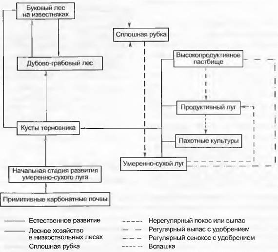
Regressive successions lead away from climax vegetation and are associated with its degradation. Barring natural disasters (earthquakes, storms, etc.) or catastrophic biological events (such as Dutch elm disease, see Ophiostoma), they are almost invariably a reaction to human intervention (see Fig. 13.51). The most severe disturbances are those that damage soils either directly or indirectly by weakening the vegetation cover (overgrazing, regular burning).

Natural and anthropogenic vegetation shifts on the limestone soils of the lower mountain zones in Central Europe exhibit both progressive and regressive trends which, although cyclically interconnected (Fig. 14.38), remain reversible. However, regressive shifts leading to soil degradation—such as overgrazing and increased fire frequency on stony heathlands that drive the degradation of Mediterranean oak forests—are largely irreversible.

14.3.3. Classification of Vegetation Types

Although the biocoenoses comprising the biosphere form a continuum, distinct boundaries nevertheless emerge between different plant communities due to spatial variations in habitat conditions and differences in successional stages. Within vegetation systematics, the typification of specific plant communities is both feasible and useful. Statistical analyses also demonstrate that only very specific combinations of species tend to co-occur (Fig. 14.39). These characteristic species groups can be delineated as abstract vegetation types that are realistically demarcated from one another. On an aerial photograph of an undisturbed wetland forest landscape in Alaska (Fig. 14.40), the various vegetation units mapped can be readily distinguished even by eye. Within the transition zone (ecotone), the species composition changes quite rapidly, whereas within a given vegetation type it fluctuates very little.

Fig. 14.39. Co-occurrence frequency of 43 meadow species (circles, letter symbols) in the Netherlands, presented as a diagram of synecological correlations (visualize in 3D!). Different species frequently grow together (thick connecting lines) and characterize specific plant communities (and thus habitats), such as wetland meadows with purple moor-grass = Molinia caerulea (М) and tawny sedge = Carex panicea (Ср), tormentil = Potentilla erecta (Ре), dissective thistle = Cirsium dissectum (Cs), etc.; marshy riparian reed beds with reed canary grass = Phalaris arundinacea (Pha) and reed sweet-grass = Glyceria maxima (Gm), lesser tussock sedge = Carex disticha (Cd), marsh marigold = Caltha palustris (Cal), etc.; nutrient-rich hay meadows with false oat-grass = Arrhenatherum elatius (Arr) and orchard grass = Dactylis glomerata (D), golden oat-grass = Trisetum flavescens (Tn), etc.; intensively managed pastures with perennial ryegrass = Lolium perenne (Lp) and crested dog's-tail = Cynosurus cristatus (Су), annual meadow grass = Poa annua (Ра), red clover = Trifolium pratense (Тр), etc.

Fig. 14.40. Comparison of an aerial photograph (A) and a vegetation map (B) (lowland north of Anchorage, Alaska; area 400 × 370 m): a — mixed birch forest (Betula resinifera, etc.) outside wetlands and river floodplains; b — floodplain mixed forest with balsam poplar (Populus balsamifera) and birches; c — riverbanks with willow scrub (Salix sp.); d — boggy spruce forests (Picea mariana); e — mossy dwarf-shrub heaths (Vaccinium uliginosum, Ledum decumbens) and Sphagnum; f — sedge-dominated marshy meadows (Carex, Eriophorum, etc.); g — water bodies and sandy shoals

In the floristic classification of vegetation, species are grouped according to their degree of similarity into hierarchically subordinate units (species assemblages). These groups of species with similar environmental requirements constitute habitat-typical plant communities. Typically, such communities contain dominant or highly typical species (characteristic or faithful species) that can be used to name the community. This principle underlies the Zürich-Montpellier (Braun-Blanquet) syntaxonomic system of plant communities, which has become an essential tool for geobotanical mapping and synthesis (Table 14.4), particularly in Europe.

Table 14.4. Syntaxonomic System of Plant Communities

Thus, associations of the ryegrass meadow alliance belong to the class of European sown meadows and are subdivided into specific facies according to their subunits: with Molinia, with Arrhenatherum, with Briza, with Salvia, and with Bromus erectus.

Associations and alliances are primarily used as conventional syntaxonomic units (e.g., Fagetum, Abietetum, Pinetum for beech, fir, and pine forests, respectively). Linguistically, associations are designated by the suffix -etum (a Latin collective suffix) appended to the root name of the dominant genus. For instance, a larch-pine forest is termed Larici-Pinetum, and a heather-pine woodland is termed Erico-Pinetum.

The syntaxonomic characterization of a given plant community relies upon:

• characteristic (faithful) species — species whose primary distribution area is restricted to one of the major taxonomic categories (characteristic species of an association, alliance, order, or class) and which characterize it particularly well from a floristic standpoint;

• differential species — species that best separate one syntaxon from another closely related one, without being strictly confined to that syntaxon, as they may also occur in other, more distantly related classification units.

Characteristic species of mixed broad-leaved forests (class Querceo-Fagetea) include Daphne mezereum and Anemone nemorosa; for the order Fagetalia, examples are Ranunculus ficaria and Mercurialis perennis; and for the alliance Fagion, they are Cardamine (= Dentaria) bulbifera and Hordelymus europaeus.

The high degree of habitat overlap among certain species groups (see Fig. 14.39) allows for the ecological characterization of these habitats, meaning that species can frequently serve as environmental indicators. It is rare to have measured ecophysiological characteristics available for every species. Nevertheless, drawing on the accumulated expertise of generations of field botanists, specific properties can be attributed to individual species. Indicator value tables (such as the Ellenberg or Landolt systems) represent a semi-quantitative method of this kind. In these systems, indices ranging from (0)1 to 9(10) are assigned to species according to their characteristic responses to specific available environmental resources, with values increasing along a gradient. A high moisture index indicates that the occurrence of the species correlates with high soil humidity. Typical indicator plants for strongly acidic soils (R from 1 to 2, see below) include Deschampsia flexuosa and Vaccinium myrtillus. While this index does not express a causal relationship regarding the species' physiological requirements, such a relationship can often be inferred. These indicator values are valid not for isolated individual organisms, but for plants growing within a community and engaging in biotic interactions. An additional challenge is that, for purely practical reasons, this method is tied to the species level as a whole; yet ecotypes of a single species may differ in their ecological requirements even more than two distinct species. Despite this, such rating Methods are of immense practical importance primarily due to their simplicity and, quite remarkably, their accuracy (Table 14.5).

Table 14.5. Ellenberg Indicator Values for Central European Conditions

Plant species with similar combinations of code numbers form an ecological group. The average values of these numbers allow for an Assessment of the entire plant community, with indifferent species (those not bound to a specific community) being excluded in advance, and only typical species taken into account,

"weighted" according to their cover values. This list is expanded by incorporating any other significant indices, making it possible to perform diverse analyses within a database framework. For instance, one can add data on morphology (life forms), dispersal mechanisms, flowering time, sensitivity to disturbances (e.g., ruderal vs. non-ruderal species), hemeroby ("culture-dependence," indicating conditions unaltered by anthropogenic impacts), time of Introduction into the flora (autochthonous species, neophyte), as well as phytogeographical data (distribution range).

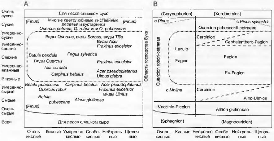
Vegetation units of a higher rank than the alliance are too abstract and therefore less suitable as examples of specific plant communities. In Fig. 14.41, Central European forest plant communities are presented in a coordinate system relative to moisture and soil reaction, with individual characteristic species shown on the left for comparison with The system of syntaxa presented on the right.

For all vegetation complexes—i.e., combinations of multiple communities—vegetation classification under a similar nomenclature is developed by sigma-sociology (symphytosociology), which is primarily applied in German-speaking countries (sigma Σ denoting the sum sign). Because certain species naturally combine with one another into communities, different communities must be grouped together (for example, a forest clearing, a forest, and a streamside form a complex that constitutes a single entity, a "sigmetum"). By analogy with syntaxonomy, sigma-syntaxonomy employs The concepts of characteristic and differential species for community sigmeta and uses endings corresponding to the J. Braun-Blanquet system.

Fig. 14.41. Forest-forming tree species of Central Europe: A — characteristic species for soils ranging from acidic to alkaline (nutrient-poor and nutrient-rich, respectively) and from moist to dry (in the submontane mountain belt and under moderately suboceanic climatic conditions). Approximate quantitative ratios within near-natural community assemblages are italicized (names in parentheses apply only to certain regions); B — phytosociological system of Central European deciduous forest communities on soils ranging from acidic to alkaline (nutrient-poor and nutrient-rich, respectively) and from wet to dry (in the submontane mountain belt and under moderately suboceanic climatic conditions). The marginal zone features spruce (Vaccinio-Piceion) and alder (Alnion glutinosae) forests; non-forest vegetation types include xerophytic grasslands on nutrient-poor and lime-rich substrates (Corynephorion and Xerobromion, respectively), as well as raised bogs (Sphagnion) and overgrown shoreline communities (Magnocaricion). Boundary lines in nature correspond to zones with transitional types of community assemblages

14.3.4. Physiognomic Classification of Vegetation Cover

Regardless of their floristic composition, plant stands can be grouped according to dominant life forms and physiognomic features (habit, external appearance). Such vegetation types, characterized as independent yet essentially complex entities, are termed formations; examples include tropical rainforests, boreal coniferous forests, evergreen sclerophyllous shrublands, dwarf-shrub heaths, and meadows. Conversely, simple plant assemblages composed of only a single life form that often do not exist independently are designated as sinusia—for instance, the crust of crustose lichens on rocks, the dwarf-shrub layer in a coniferous forest, or the assemblage of cap fungi in an autumn deciduous forest. Plant formations, together with their surrounding environment, form biological formations, or biomes for short. They are named after the dominant plant formation; hence, biomes and formations are synonymous in nomenclature.

There are undeniable overlaps with the syntaxonomic division of vegetation. Despite differences in species composition, identical genera often grow within similar biomes; for example, in the summer-green deciduous forests of cold-winter temperate regions in North America and Eurasia, these include the genera Quercus, Fagus, Carpinus, Acer, Tilia, and others. Conversely, convergent physiognomic similarities are observed in formations composed of representatives from different families, driven by similar environmental conditions. Examples include the sclerophyllous shrublands of the Mediterranean climate distributed globally, or the series of succulent semi-deserts in the Old and New Worlds (Euphorbiaceae — Cactaceae). Some formations are almost independent of the climate of their Location, such as grasslands that thrive in both continental temperate steppe regions and the tropics.

An attempt to classify the vegetation cover of the Earth's entire land surface into formation types (considering only late successional stages) is presented in Fig. 14.42. The coordinates represent mean annual precipitation and mean annual temperature, with the latter, as seen in the climadiagrams, reflecting potential evapotranspiration. Individual formations are described in more detail in Chapter 15.

Fig. 14.42. Continental formations: an attempt to classify climax vegetation based on mean annual temperature and precipitation. Symbols indicate characteristic life forms. Boundary lines are fuzzy, especially in the central part of the diagram, as the relative positions of formations in relation to climatic data can shift quite significantly across different regions

14.3.5. Spatial Structure of Vegetation and Biotopes

Within a given regional climate, relief- and edaphic-conditioned horizontal zonation of natural vegetation (or its fragments) emerges, intertwining with human-impacted vegetation (cultural landscape). Often, actual (anthropogenic) vegetation differs markedly from potential natural vegetation (e.g., pastureland in place of a forest). Vegetation maps depict this spatial zonation of the plant cover. However, they can only display plant communities at the association rank on a very large scale. Regional or, even more so, interregional maps can only represent broad vegetation complexes, as illustrated by the map of Lower Austria in Fig. 14.43. Maps of this or an even smaller scale generally represent only potential vegetation—that is, the vegetation that could persist over the long term in the absence of human impact. On a continental or global scale, the spatial structure of vegetation corresponds to major climatic zones driven by decreasing temperatures from the equator to the pole, overlain by the oceanicity-continentality gradient. At such a scale, only climax formations of potential vegetation are displayed.

Fig. 14.43. Division of the Central European vegetation cover using Lower Austria as an example. Potential natural climax vegetation (forests almost everywhere!), corresponding altitudinal belts, and large areas of long-term derivative plant communities. Floristic regions (subregions) among zonal vegetation types: 1–2 — Pannonian, 3–8 — Central European, 9–13 — Alpine. Floodplain forests (20) are present along major rivers (Danube, March, etc.)

When delineating altitudinal vegetation belts in mountains, we are also dealing with vegetation complexes that in each case correspond to the dominant potential climax formation or dominant plant community (Fig. 14.44). The succession of these vegetation complexes reflects the climate changing with increasing elevation ("altitudinal" climate). The only climatic feature common to all zones along the altitudinal gradient is the drop in temperature. All other climatic factors vary depending on latitude (the shortening of the vegetative period with elevation is a phenomenon restricted to extra-equatorial latitudes) or regional macroclimatic peculiarities (in some areas of the Earth, cloud cover, precipitation, or wind increases with altitude, while in others they decrease). Strong differences are also observed between the marginal zones of mountain systems and their inner, mostly more continental parts, as well as between windward and leeward mountain ranges relative to the prevailing air mass direction. International standard designations for mountain belts and their corresponding vegetation succession in the Alps are given in Fig. 14.44. Middle and low mountain, foothill (hilly), and lowland belts also exist.

Fig. 14.44. Upper altitudinal belts of the Alps with characteristic mosaic-structured formation complexes

Unfortunately, The Use of this altitudinal belt nomenclature in literature is not always uniform. This primarily concerns the term "subalpine," which is used in a very broad sense. This interpretation, shown in Fig. 14.44, is the most widely adopted worldwide and encompasses the zone where upper-belt mountain woodlands intermingle with alpine vegetation (often referred to as the treeline ecotone). Nevertheless, regional "schools" also use this term from a phytosociological standpoint to designate the belt of mountain forests (upper subalpine belt). The terms "nival" and "subnival" are rarely used outside of Europe. The term "alpine" applies not only to the Alps (the root alb, alp, or alpo appears in words denoting mountains or their slopes in Latin, and possibly in Proto-Indo-European; see Ch. Körner, 1999) but is also used globally to designate treeless vegetation located above the natural climatically determined timberline (even where it is locally absent due to anthropogenic impact or natural disturbances). The colloquial use of "alpine" simply in the sense of "mountainous" ("alpine landscape," "alpine economic region," "alpine culture") has nothing in common with its phytogeographical definition. In the Andes, the term "andean" is used for the alpine belt, while in Africa, "afroalpine" is used.

14.3.6. Correlative Analysis of Vegetation

Based on the vegetation inventory and its classification described in Section 14.3.3, combined with data on habitat characteristics and indicator

species, a series of ordination and correlation analyses can be performed, the ultimate goal of which is to reveal recurring patterns in the distribution of species and plant communities and to explain them based on specific environmental conditions.

Gradient analysis focuses on vegetation changes driven by shifting environmental conditions. Ideally—though this is far from always the case—a single coupled gradient is realized within the studied plots. When ordering species abundance along environmental gradients, for instance, they are sorted by increasing or decreasing gradient values, a process known as direct ordination. If only a single variable is chosen, this is a univariate ordination (a clear example being the vegetation profile along a transect from the seashore according to soil salinity, see Fig. 13.28). A two-dimensional representation is referred to as an ecodiagram (see Fig. 14.42), where The values of two environmental parameters are plotted on two axes, and the habitat of a plant species or community is assigned a specific coordinate value in an X–Y system representing THE POSITION OF the species or community in a two-dimensional space (Figs. 14.45, 14.46). This generates patterns (e.g., clusters, correlations) that can be interpreted as preferred habitat conditions for specific associations. Because environmental factors typically act simultaneously, making it unclear which single factor or combination thereof is critical, ordination space in detailed analysis is invariably multidimensional and can only be comprehended using computational methods. Consequently, this is referred to as correlative (as well as mathematical, numerical, statistical, multivariate, or quantitative) vegetation analysis.

Fig. 14.45. Beech forest types (1–38) ordered by their co-occurrence in Fagetum associations in France using optimal two-dimensional factor analysis. Gradients include moisture and soil fertility. Indicator species groups for nutrient-rich (A), fresh (B), nutrient-poor (C), and typical (D) communities are clearly identified

A large number of multivariate methods and calculation software have been specifically developed for vegetation parameters combined with habitat data (e.g., correspondence analysis CA, canonical correspondence analysis CCA, and alternatively Principal Component Analysis PCA). As a rule, this analysis is carried out in two stages. First, the vegetation type is "identified" and determined, and then the environmental parameter values are determined for it, or more precisely, for individual vegetation relevés. Both stages are based on correlation analysis. This makes it evident which environmental factors are most likely to determine vegetation patterns.

Fig. 14.46. Plant communities of Poland ordered by their floristic similarity using optimal two-dimensional polar ordination: raised bog (Sphagnetum medii = Sm), wooded bog (Pineto-Vaccinietum uliginosi = PVu), pine forest (Pineto-Vaccinietum myrtilli = PVm), fir forest (Abietetum polonicum = Ap), caricetum elongatae alder swamp (Cariceto elongatae-Alnetum = CeA), ash-alder floodplain forest (Circaeo-Alnetum = CA), oak-hornbeam forest (Querceto-Caprinetum medioeuropaeum = QC), beech forest (Fagetum carpaticum = Fc), mixed oak forest (Querceto-Potentilletum albae = QP), hazel scrub (Coryleto-Peucedanetum cervariae = CP). The numbers in parentheses after each community indicate the mean number of vascular plant species

Each of the plant communities in the study area becomes an "object" ("component") characterized by its species composition (= "attribute"). The occurrence of a species in a particular plant community serves as its specific feature, just as the prevailing environmental conditions constitute a feature of that species, determined In the second stage. Such correlation methods typically do not rely on a simple presence-absence determination ("yes or no"), but rather record species by taking their abundance into account (see 14.3.1). Therefore, each species is assigned a conventional abundance axis starting from zero and ending at 5 (100% cover). Each vegetation relevé is positioned along this axis depending on how abundant the species is within it. Because There are many species (and abundance scales), a multidimensional (correlation) space arises, in which individual vegetation relevés are simultaneously subordinated to many axes of individual species. While this is almost impossible to visualize mentally, it is well-suited for mathematical Processing. Each vegetation relevé (each object) corresponds to a point in this complex multidimensional coordinate system. If 100 relevés are processed, there will be 100 points. Using mathematical methods, this multidimensional system can be reduced to a few axes, and the cloud of points (relevés) can then be represented in a two- or three-dimensional space. In the process, the multidimensional system is compressed so that the major part of the floristic diversity is reflected on a few axes. Species assemblages (vegetation relevés) are thus ordered relative to one another into a diagram based on their floristic similarity (distance within the diagram). Such a diagram reflects groups of relevé clusters (objects). These correspond to community types, and the method fulfills the requirements of non-hierarchical classification. The point clouds of a cluster are immediately recognizable either as sharply delimited groups (= vegetation types) or as transitioning into one another more or less gradually.

If, instead of vegetation relevé numbers, the corresponding pH values, soil types, moisture levels, topographic positions, etc., are plotted in the correlation space, the correlation between species abundance and habitat conditions can be established in the same way. Changes in habitat conditions among different relevés indicate environmental gradient directions (e.g., lower pH values on the left side of the axis, higher values on the right). Rotating the coordinate system also reveals a position where one of the axes achieves maximum dispersion of "loadings" (the "first" axis holds the greatest significance for subsequent interpretation). If a specific gradient lies parallel to the first axis, it can be inferred that this particular ecological factor exerts the strongest influence on the species composition. The second axis, positioned at a right angle to the first, displays the highest remaining dispersion, i.e., the next most important factor, and so on. This "indirect gradient analysis," supported by specialized computer software, allows for the processing of very large datasets.

Component analysis is likewise a process of reducing spatial dimensions by projecting multidimensional point clouds into a two- or three-dimensional space. The resulting axes are an outcome of the analysis rather than being established a priori, as is the case in one- or two-dimensional (graphic) ordination. In this way, it is possible to determine under what environmental conditions two species can co-occur with high abundance (i.e., to establish their shared habitat preference). This can be achieved using computer software through a comparative Analysis of the entire species composition, from which a matrix of relationships (a network of correlation pleiades, a raster diagram, see Fig. 14.39) is calculated and constructed. Such similarity analysis is used in the numerical classification of closely related plant communities and is subsequently represented as a dendrogram (cluster analysis).