Biological Membranes - A. N. Ogurtsov 2012

Electrogenesis of Biomembranes
Nonequilibrium Thermodynamics of Biomembranes
Flux Coupling in Biomembranes

An Organism or a Cell is a chemical machine that Functions through Chemical Reactions and the Transport of substances between The Cell and its environment, as well as within the cell itself. This transport has a specific direction perpendicular to the outer Cell Membrane and intracellular Biomembranes.

The flux of matter is a vector quantity, whereas The rate of a chemical reaction is a scalar. According to the Curie-Prigogine principle, direct coupling between scalar and vector processes is impossible in an isotropic medium. However, biomembranes are fundamentally anisotropic systems composed of molecules lacking a plane and a center of Symmetry. It is this membrane anisotropy that makes it possible to couple scalar and vector processes—specifically, linking mass transport with chemical reactions. The presence of membranes ensures the compartmentalization of biological systems. A biomembrane acts as a barrier that maintains differences in environmental parameters across its opposing sides, thus establishing a jump in a given system parameter (such as the concentration of a specific component or an electrical potential) across the membrane.

Let us first consider an example where an aqueous sucrose solution is placed in two compartments, A and B, separated by a membrane M (Figure 166).

Class="center">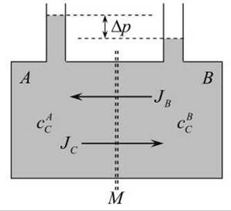

Figure 166 - Passive transport of substances across membrane M

The membrane is partially permeable to sucrose molecules and fully permeable to Water molecules (the solvent). As a result, two fluxes are established across the membrane: sucrose flux J_C and water flux J_B. The dissipation function for these two fluxes is given by

Under isothermal conditions, the driving force for both fluxes has the form

where ∆p is the hydrostatic pressure difference between the two compartments, ∆μ is the difference in the chemical potentials of the substance on both sides of the membrane, and is the partial molar volume of the substance. Then

or

The difference in chemical potentials ∆μ_с is related to the osmotic pressure μπ, which compensates for the difference in solution concentrations on both sides of the membrane. According to the van 't Hoff law,

For the chemical potential,

at dμ⁰ = 0. For the example under consideration, let us express ∆μ_с in terms of a small increment of the chemical potential

where is the average concentration of sucrose in the system

Consequently,

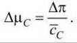
The relationship between the two coupled fluxes—the solute and the solvent—obeys the Gibbs-Duhem equation

Consequently,

Taking this into account, the dissipative function takes the form

Thus, the dissipative function is represented by new generalized forces (A_p and A_D) and new flows

where J_p is the volume flow; J_D is the diffusion flow. Now

For the coupled flows J_p and J_D, in accordance with the equations

we can write

Let us determine the physical meaning of the phenomenological coefficients.

First, let us consider the situation where the sucrose concentration is the same on both sides of the membrane, c_A = c_B. In this case, Δπ = 0. Consequently,

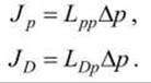
Thus, the difference in hydrostatic pressure induces a volume flow J_p and an additional diffusion flow J_D, which leads to the redistribution of sucrose.

This phenomenon is called ultrafiltration, and the coefficient L_Dp is referred to as the ultrafiltration coefficient.

Second, let us consider the case where the hydrostatic pressure is the same on both sides of the membrane, i.e., Δp = 0, then

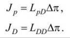
The coefficient L_DD is called the solute permeability coefficient through the membrane.

The additional volume flow J_p is termed the osmotic flow, and the coefficient L_pD is called the osmotic flow coefficient. Using the Onsager reciprocal relation L_ij = L_ji, we obtain the relationship between the flows

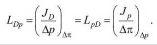
Now let us consider the situation where the volume flow J_p = 0. Then

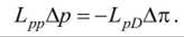
Let us introduce a new constant k, which is called the reflection coefficient (Staverman constant)

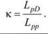
The reflection coefficient k depends on The properties of the membrane. Let us express the volume flow taking k into account

Let us consider two hypothetical extreme scenarios. If k = 1, the solute does not penetrate the membrane at all (it is completely "reflected" by the membrane), and therefore

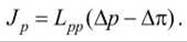
If k = 0, the membrane is fully permeable and

The reflection coefficient k characterizes The Mechanism of solute Transport Across the membrane. It equals zero when L_pD = 0, which means there is no coupling between the J_p and J_D flows—meaning solvent transport occurs independently of solute transport. In real-world conditions, k ≤ 1 and L_pD≠ 0, indicating a coupling between the J_p and J_D flows. This is a crucial detail that is frequently overlooked when WATER AND SOLUTE transport processes into the cell are (erroneously) treated as independent. Only by applying the principles of Linear Nonequilibrium Thermodynamics and utilizing the Onsager reciprocal relations to transport phenomena across The cell membrane can we quantitatively and accurately describe The transport of substances into the cell.

It should also be borne in mind that Introduction/36.html">Biological Membranes differ fundamentally from artificial, non-biological semipermeable membranes (such as porous rubber partitions separating two liquid phases) due to the presence of facilitated and Active Transport processes, which can only be described using the Methods of nonequilibrium thermodynamics.

For instance, the Nа⁺/К⁺-ATPase drives the simultaneous transport of sodium and potassium ions across the membrane. We can single out the "exchange" force

which describes the total Ion Exchange across the membrane. The net exchange flow J_обм indicates that K⁺ ions are exchanged for Na⁺ ions.

The remaining (r, rest) coupled forces Х_r drive the chemical flows Jr. Consequently, the local Entropy generation inside the membrane is given by

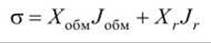
and, accordingly, in the linear approximation

By definition, in active transport, the flow J_oбм is directed against the action of the forces J_oбм. This is only possible when the coefficients L₁₂ = L₂₁ are non-zero.

Indeed, according to the condition L_іі > 0, the coefficient L₁₁ must be positive. Therefore, if L₁₂= 0, it follows from J_обм = L₁₁X_обм + L₁₂X_r that J_обм and J_обм must have the same sign, making active transport impossible. Conversely, if the coupling term L₁₂X_r takes on negative values, the direction of the flow J_обм is reversed against the force J_oбм.

From the equation σ = X_oбмJ_oбм ⁺ X_rJ_r, it is evident that active transport makes a negative contribution to entropy generation, thereby reducing its value. Without the coupling of various flows and forces, processes leading to a decrease in entropy would be impossible.

Let us examine two processes occurring in vesicles containing a proton pump (H⁺-ATPase): J_H, the proton (H⁺) flow, and J_р, the ATP Hydrolysis, which can be represented as:

where Х_Н = ∆μН⁺; L_РН = L_HР; Х_р is The change in Free energy during ATP Cleavage. The chemical energy of ATP hydrolysis J_pX_p is transformed into the energy of proton transport J_HХ_H.

Let us introduce the transformation coefficient η, which, given the condition Ф = J_HX_H + J_pX_p > 0, is equal to

If we define the dimensionless quantity

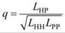
- is the degree of coupling, where -1 < q < 1 (with q = 1 indicating 100% transformation of chemical energy into another form of energy). It can be shown that the maximum transformation efficiency is given by

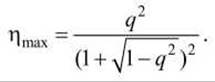
Since any system experiences energy losses, the value of q must be less than 1.

If X_H increases in the presence of proton transport, the value of η decreases. While in closed systems the coupling coefficient between standard reactions is expressed by integers, in open systems—such as Oxidative Phosphorylation in biomembranes—the coupling between oxygen consumption and phosphorylation processes is represented by a fractional number.

As mentioned earlier, any open system in general (and biomembranes in particular) can maintain a stationary, albeit non-equilibrium, state.

This state is characterized by a constant entropy value. A living organism persists in this state provided that as certain parameters change, others remain constant.

In our example, the change in entropy with respect to volume, taking into account L₁₂ = L₂₁, will be

where the force X₂ is denoted by a fixed value X⁰₂ = const. Differentiating this expression with respect to X₁ gives

whence

represent constant values proportional to X⁰₂.

In other words, in a stationary state close to equilibrium, the entropy change is minimal. This state is analogous to The equilibrium state in closed systems. As previously noted, the coupling of various fluxes can drive processes characterized by a negative entropy change in other pathways.

This phenomenon of compensating for a negative-entropy flux is one of the essential conditions for sustaining the vital activity of an organism.