Biological Membranes - A. N. Ogurtsov 2012

Electrogenesis of Biomembranes
Nonequilibrium Thermodynamics of Biomembranes
Linear Nonequilibrium Thermodynamics

If n forces act in a system, producing n flows, determining the functional dependence between them requires the experimental evaluation of n x n phenomenological coefficients.

In reality, the number of independent phenomenological coefficients is smaller; this reduction can be attributed to the following reasons.

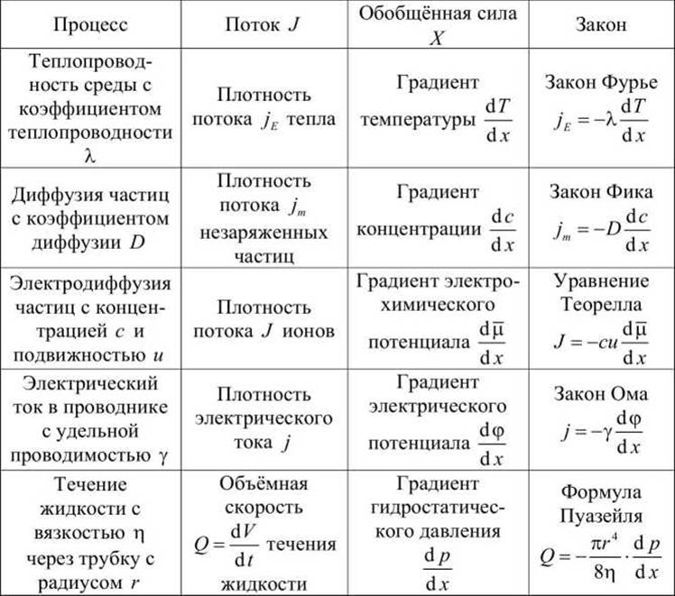
First, the Symmetry of the system plays a role—in the case of a symmetrical isotropic medium, every flow does not necessarily need to couple with all forces,

Class="center">Table 6 - Examples of linear irreversible processes

Second, Onsager's theorem, or the Onsager reciprocal relations, holds true—the phenomenological coefficients form a symmetrical matrix, i.e.,

Third, the uncoupled (i = j) coefficients are always positive

Lu > 0.

Indeed, let us consider a system involving only two flows, for example, heat q and matter d, then

Since

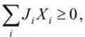
then

Suppose further that the Temperature gradient vanishes while only the concentration gradient remains, i.e., X_q = 0, X_d≠ 0, then and consequently, L_dd > 0. Similarly, by leaving only the temperature gradient, it can be shown that L_qq > 0. Furthermore, (L_qd + L_dq)² < 4L_qqL_dd, which implies

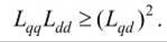
In the general case for linear systems with an arbitrary number of forces and flows, it can be demonstrated that and

Let us formulate (without proof) a few more fundamental principles of linear nonequilibrium Thermodynamics.

As mentioned above, The Second Law of thermodynamics requires the condition 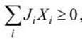to be satisfied, which applies to the sum as a whole.

Individual terms of this sum can be negative. This means that an isolated, individual flow J_i with J_iХ_i < 0 is impossible, as it contradicts the second law of thermodynamics. However, through coupling with other flows J_j, for which J_jX_j > 0, an open system can sustain a flow that would be unthinkable in an isolated system. The only requirement is that the condition

Flow coupling is determined by the non-zero values of the off-diagonal coupling coefficients L_ij.

For instance, a binary gas mixture in a vessel whose walls are maintained at different temperatures spontaneously separates such that the concentration of one gas is higher near the hot wall and the other near the cold wall. This phenomenon is known as thermal diffusion. The matter flux moves in the direction opposite to the concentration gradient because it is coupled with the heat flux flowing from the hot wall to the cold wall. The Entropy deficit in one process is offset by its excess production in the other.

We can see that entropy production in an open system fundamentally enables processes that are impossible in isolated systems. This is crucially important for understanding endergonic processes in biological systems.

The coupling of Chemical Reactions in an open system makes endergonic reactions possible (reactions in which the Free energy of the system increases), which are prohibited in isolated systems.

For example, The formation of each peptide bond during Protein Synthesis is accompanied by the release of one Water molecule. Since water is present in excess within The Cell, the reverse reaction—the Hydrolysis of peptide bonds—should normally predominate. The synthesis of a polypeptide chain becomes possible due to the coupling of the synthesis reaction with the exergonic Cleavage (hydrolysis) of ATP, and the dissipation function as a whole remains positive.

The Coupling of Endergonic processes with ATP hydrolysis is of general biological significance. Through this coupling, the universal role of ATP is realized as a donor of the free energy required to drive endergonic processes. If Cells and organisms were isolated systems, ATP could not perform this function.

Nonequilibrium thermodynamics proves, already within the linear approximation, that processes prohibited in isolated systems can occur in open systems. This is of fundamental importance for biology.

The Curie-Prigogine principle. Flows and forces can be either scalar or vector quantities. In an isotropic system (a system whose properties are identical in all directions), a constraint is imposed on the coupling of flows, known as the Curie-Prigogine principle. Its core meaning is that coupling between scalar flows (e.g., chemical reactions) and vector flows (e.g., matter fluxes, heat flows) is impossible—a scalar cannot be the cause of a vector, nor can a vector be the cause of a scalar (a force cannot cause a flow of a different tensor dimension).

Another formulation of this principle states that external influences giving rise to various phenomena cannot possess a higher symmetry than the effect they produce.

The Curie-Prigogine principle also holds true for an anisotropic system that possesses a center of symmetry in its equilibrium state. In all other cases of anisotropy, as well as in the nonlinear region (when the deviations of the system from The equilibrium state cannot be considered small and nonlinear terms of the Taylor series cannot be neglected)—where the property of isotropy disappears regardless of the medium's Structure at equilibrium—the Curie-Prigogine principle is not applicable.

Prigogine's theorem. An open system can exist in a stationary, albeit nonequilibrium, state. In this state, entropy production within the system is exactly balanced by the efflux of entropy into the surroundings, so that the total entropy of the system remains constant

Such a stationary state is referred to as a steady-state equilibrium.

A visual model of this state is shown in Figure 165.

Figure 165 - Model illustrating the steady-state equilibrium of an open system: a - closed system, b - model of an open system

The liquid level in the intermediate vessel will settle at a certain position determined by how wide the Valves connecting the vessels are open. By adjusting the valve settings, new liquid levels can be established—representing a new stationary state of steady-state equilibrium.

The stationary state of an open system is realized if constraints are imposed on the system that fix constant values for a portion of the generalized forces, while the remaining generalized forces are allowed to vary.

For example, let two generalized forces X₁ and X₂ act within the system, with the first one being fixed as X₁ = const (for instance, the first force represents a fixed temperature gradient that does not change).

As shown above, entropy production is described by the relation

Since L₂₂ > 0, the second derivative with respect to X₂ (at X₁ = const) is

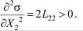
Consequently, Prigogine's theorem holds in the stationary state: In a stationary state close to equilibrium, the entropy production σ is at a minimum.