Fundamentals of Bioinformatics - Ogurtsov A.N. 2013

Methods of Bioinformatic Analysis
Sequence Alignment Algorithms
Global Alignment Algorithm

The Needleman-Wunsch global sequence alignment algorithm using dynamic programming relies on constructing the optimal alignment at The current stage by using the optimal alignments of the initial fragments of the original sequences obtained in previous steps.

For two sequences to be aligned, x and y, with elements x_i (0 < i < n) and y_j (0 < j < m), we construct a matrix F.

The element F(i, j) of this matrix contains the score of the best alignment of the initial fragments x_1...i (of length i) and y_1...j (of length j) of sequences x and y, respectively. Matrix F is constructed recursively. We start by assigning a zero score to the starting point: F(0,0) = 0. Next, we fill in the matrix in order of increasing indices, that is, from the top-left corner to the bottom-right. Once F(i - 1, j - 1), F(i - 1, j), and F(i, j - 1) are known, F(i, j) can be calculated.

There are three possible ways to obtain the score F(i, j), corresponding to the three possible alignment scenarios shown in Figure 49.

Class="center">

Figure 49 - Three ways to extend the alignment to a point: a - element x_i is aligned with y_j; b - element x_i is matched with a gap; c - element y_j is matched with a gap

An element x_i of the first sequence can be aligned with an element y_j of the second sequence (Figure 49(a)), in which case the alignment score s(x_i, y_j) (e.g., from a BLOSUM matrix) is added to the score F(i - 1, j - 1)

F(i, j) = F(i - 1, y - 1) + s(x_i, y_j).

If an element x_i of the first sequence is aligned with a gap In the second sequence (Figure 49(b)), a penalty d is "assessed" for this

F(i, j) = F(i - 1, j) - d.

When an element y_j is aligned with a gap in sequence x (Figure 49(c)), a penalty is likewise "assessed"

F(i, j) = F(i, j - 1) - d.

The maximum alignment score for two sequence fragments x_1...i (of length i) and y_1...j (of length j) is determined as the maximum of these three options

This recursive Procedure is repeated by sequentially increasing the row index j (and, within each row, sequentially increasing the Column index i) until the entire matrix F(i, j) is filled.

Let us consider a "square" consisting of four adjacent Cells of the matrix (Figure 50).

Figure 50 - Three ways of obtaining the score F(i, j)

Each subsequent value of F(i, j) in the bottom-right corner of such a four-Cell "square" is determined from one of the other three cells (indicated by arrows in Figure 50).

When filling the matrix F, alongside calculating The values of F(i, j), it is necessary to record which of the three "paths" (from which cell in Figure 50) this specific value of F(i, j) was obtained.

Such tracking is subsequently required, after the entire matrix is filled, to reconstruct the optimal "traceback" path.

Before completing the Description of the algorithm, we must define the boundary conditions—the procedure for filling the cells of the top row (j = 0) and the left column (i = 0).

Since along the top row, where j = 0, obtaining the values F(i, 0) by moving from left to right (the horizontal arrow in Figure 50) corresponds to inserting gaps into sequence y, we set

F(i, 0) = -d.

Similarly, along the left column where i = 0

F(0, j) = -d.

Let us consider The process of filling the dynamic programming matrix using the global alignment of two sequences as an example

using the BLOSUM50 substitution matrix and a gap penalty value of d = 8.

First, following the rule for filling the top row (y = 0) and the left column (i = 0), we fill the corresponding cells of the dynamic programming matrix with cumulative penalties (Figure 51) and mark the "path" of cell filling with arrows.

Next, we begin filling the row with j = 1. For cell (1,1), i.e., for The amino acid pair (H,P), we calculate three possible options according to algorithm (*) (p. 177) and use a pointer arrow to indicate which cell this cell was filled from

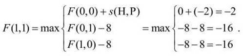
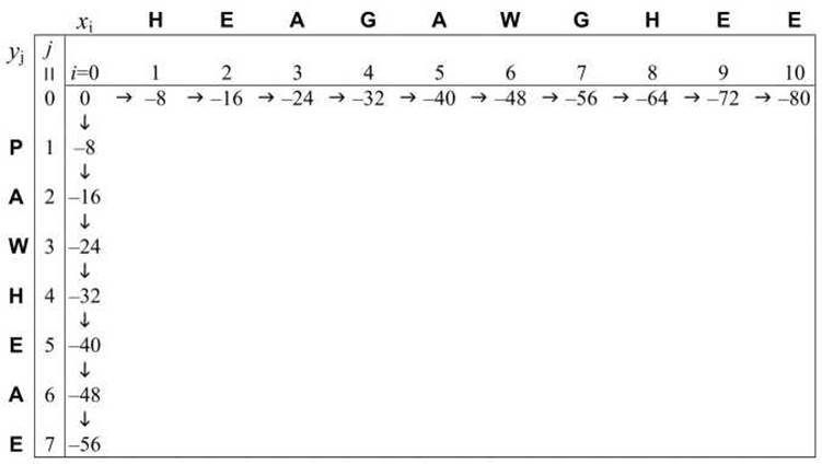
Figure 51 - Filling the top row and left column of the matrix

For cell (1,1), the maximum value is (-2) when transitioning from cell (0,0); therefore, we mark the transition from cell (0,0) to cell (1,1) with an arrow (↘) (Figure 52).

We continue filling the row with j = 1. For cell (2,1) or (E,P) of the dynamic programming matrix, we calculate three possible options according to algorithm (*) (p. 177)

and indicate the corresponding transition with an arrow (↘) (Figure 52). For cell (3,1) or (A, P) of the matrix

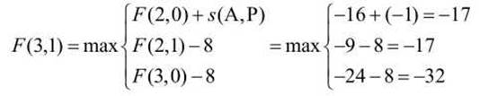
There are two identical maximum values (-17); accordingly, we mark two possible transition pathways to cell (3,1) from cells (2,0) and (2,1) (Figure 52).

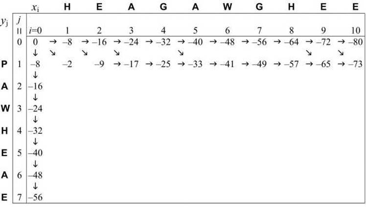
Figure 52 - Filling the row with j = 1

Next, for the remaining cells of row j = 1:

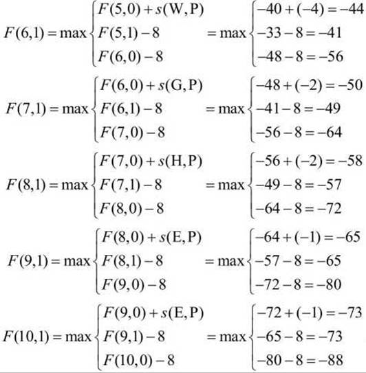
Similarly, we fill in the remaining cells of the matrix (Figure 53).

Figure 53 - Filling the dynamic programming matrix

By definition, the value of the bottom-right cell of the matrix, F(n,m), represents the optimal alignment score for the two sequences x_1...i and y_x...j. To construct the alignment itself, it is necessary to retrace The sequence of choices that led from the starting point (0,0) to the final point (n,m).

This choice-reconstruction procedure is called the traceback procedure. It is performed by building the alignment in reverse, starting from the bottom-right cell of the matrix with coordinates (n,m) and following the step pointers obtained during the matrix construction.

Figure 54 shows the traceback pointers indicated by arrows.

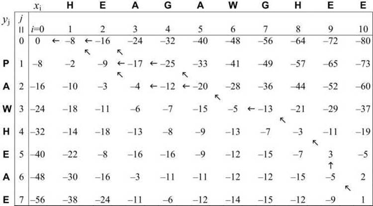
Figure 54 - Traceback scheme

At each step of the traceback procedure, we move from the current cell (i,j) "backward" to one of the cells (i - 1, j - 1), (i - 1, j), or (i, j - 1) from which the weight value F(i, j) was computed.

Simultaneously, we construct the traceback graph and record the aligned sequences by prepending a pair of characters to the current alignment on the left:

- if the weight was obtained from cell (i - 1, j - 1) (diagonal arrow);

- if the weight was obtained from cell (i - 1, j) (horizontal arrow);

- if the weight was obtained from cell (i, j - 1) (vertical arrow).

At the end of the alignment, we reach the top-left corner of the matrix (0,0).

For our example, three alternative alignment options with the same weight of 1 are possible:

The existence of multiple optimal alignments with the same weight (score) manifests as "branching points" in the traceback graph within the dynamic programming matrix. A branch occurs when the traceback procedure, which reconstructs the optimal path, reaches a cell (i, j) in the dynamic programming matrix whose optimal value F(i, j) was derived from more than one "parent" cell. This gives rise to alternative paths through the dynamic programming matrix and, consequently, different optimal alignments.

Let us consider two more representative Examples illustrating the capabilities of the global alignment algorithm.

Let us construct the global alignment of two DNA sequences: gaattc and gatta, assigning (+2) points for a match, (-1) for a mismatch, and a linear gap penalty of d = 2.

Repeating all the algorithm steps from the previous example, we obtain the dynamic programming matrix with traceback pointers (Figure 55).

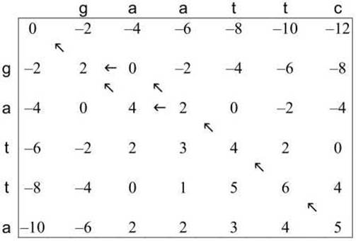
Figure 55 - Alignment matrix for the sequences gaattc and gatta

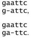
Accordingly, two optimal alignments with a score of 5 are possible:

Second example. Let us find the optimal global alignment of The nucleotide sequences tacgagtacga and actgacgactgac, subject to the condition that the NUCLEOTIDES g shown in bold must be aligned with each other. Scoring scheme: match (+2), mismatch (-1), proportional gap penalty d = -2.

It is easy to see that the middle nucleotides g divide each sequence into two identical subsequences. Therefore, if we find the optimal alignment of the subsequences tacga and actgac, the optimal global alignment satisfying the condition that the middle nucleotides g are aligned will be a concatenation of these two sub-alignments with a pair of aligned nucleotides g between them. Thus, we first compute the sub-alignment matrix (Figure 56) and use the traceback method to construct the sub-alignment itself.

Figure 56 - Alignment matrix for the sequences tacga and actgac. Alignment of the sequences tacga and actgac

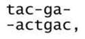
and its score is 2. The resulting global alignment has the form

and its score is S = 2 + s(g,g) + 2 = 2 + 2 + 2 = 6.

It turns out that this "conditional" optimal alignment (subject to the condition of aligned average lengths d) coincides with one of the two "unconditional" optimal global alignments of the given sequences tacgagtacga and actgacgactgac. The second optimal global alignment (with the same score of 6) has the following form

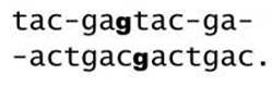
In this alignment, the two nucleotides g are not aligned with each other. However, the loss of the positive match score is compensated by a reduction in the number of gaps.