BIOLOGY Volume 2 - A Guide to General Biology - 2004

13. TRANSPORT IN PLANTS

13.1. Plant Water Relations

13.1.9. Effects of Heat and Alcohols on Membranes

Certain treatments, such as ethanol application or heating, disrupt the selective permeability of Cell membranes. Although the membranes remain intact, they behave as though breached—meaning they cease to act as a barrier to large molecules like sucrose. High temperatures and alcohols denature Membrane Proteins, while concentrated alcohols additionally dissolve Lipids.

Practical 13.2. Determining the mean osmotic potential of cell sap in plant tissue preparations using the initial plasmolysis method

The osmotic potential of plant Cells can be determined in various ways, but the initial plasmolysis method is by far the most convenient. It is based on the following relationships:

1) cell ψ = ψ₀ + ψ_p; solution ψ = ψ₀.

2) cell ψ = solution ψ when the two systems are in equilibrium.

Samples of plant tissue are brought to equilibrium with solutions of varying concentrations (having different Water potentials); the goal is to identify the solution that induces initial plasmolysis, i.e., causes the protoplasts to shrink just enough to begin pulling away from The Cell wall. At this point, the hydrostatic pressure potential of The Cell is zero because the protoplast no longer exerts pressure on the cell wall, meaning cell ψ = cell ψ₀ = solution ψ = solution ψ₀ (see equations above). In other words, the osmotic potential of the solution causing initial plasmolysis is identical to that of the Cytoplasm.

In reality, the osmotic potentials of cells within the same tissue vary, so some cells plasmolyze in more dilute solutions than others. By convention, plasmolysis is considered to begin when 50% of the cells show plasmolysis. In this case, the remaining 50% are unplasmolyzed, meaning the "average cell" is effectively at the threshold of initial plasmolysis. The resulting value represents the mean osmotic potential of the tissue.

Materials and Equipment

Onion bulb or rhubarb petiole

6 Petri dishes

6 test tubes

Test tube rack

Labels or Glass-marking pencil

2 graduated pipettes (10 or 25 ml)

2 beakers (100 ml)

Fine paintbrush

Distilled water

1 M sucrose solution

Fine forceps

Pasteur pipettes

Microscope slides and coverslips

Microscope

Graph paper

Razor blade or sharp scalpel

Procedure

Following this procedure, an alternative method using beetroot storage roots will be described.

1. Label 6 Petri dishes and 6 test tubes corresponding to the following sucrose solution concentrations: 0.3 M; 0.35 M; 0.4 M; 0.45 M; 0.5 M, and 0.6 M.

2. Using a volumetric pipette, a measuring cylinder with distilled water, and measuring cylinders with 1 M sucrose solution, prepare solutions of the concentrations listed above (see Table 13.3) and pour 20 mL of each into the corresponding test tubes.

Class="center">Table 13.3. Sucrose dilution table for experiment 13.2

3. Mix the solutions thoroughly by shaking the test tubes vigorously (this is very important) and pour them into the Petri dishes.

4. Onion. Peel off one of the fleshy scale leaves of an onion bulb. On its inner surface, cut 6 squares with sides of about 5 mm using a blade or scalpel. Using forceps, peel off the epidermal layer from these squares and place one such tissue strip into each Petri dish. Gently swirl the solution in the dishes so that it completely covers the tissue samples. Leave for 20 min.

Rhubarb. Cut 6 squares with sides of about 5 mm on the outer surface of the petiole, peel off the epidermal strips, and process them as described above for the onion.

5. Remove a tissue strip from the 0,60 M solution and use a fine brush to flatten it on a microscope slide in a drop of solution of the same concentration. Cover with a coverslip and examine under a microscope.

6. Under low power, select an area with clearly distinguishable cells. Switching to medium or high power and moving the slide, determine the state (plasmolyzed or non-plasmolyzed) of the first 100 cells encountered in the field of view. A cell is considered plasmolyzed if its protoplast has pulled away from the cell wall even slightly.

7. Repeat this procedure for the remaining samples placed in the correspondingly concentrated solutions.

8. Count the percentage of plasmolyzed cells in each solution. Plot a graph with the percentage of plasmolyzed cells on the vertical axis (ordinate) and the molar concentration of the sucrose solution on the horizontal axis (abscissa) (see Fig. 13.5).

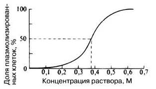
Fig. 13.5. Proportion of plasmolyzed onion epidermal cells at various sucrose solution concentrations.

9. From this graph, determine the molarity of the solution at which 50% of the cells are plasmolyzed (Fig. 13.5).

10. Using the data from Table 13.4, plot a graph showing the osmotic potential (on the ordinate) versus the molar concentration of sucrose (on the abscissa).

11. From this graph, determine the osmotic potential of the solution that causes plasmolysis in 50% of the cells. This value is considered equal to their average cytoplasmic osmotic potential.

Table 13.4. Osmotic potentials of sucrose solutions of various concentrations at 20 °C

Results

Fig. 13.5 shows a typical graph for onion epidermis. The graph for rhubarb epidermis is approximately the same.

13.5. What is the osmotic potential of onion epidermal cells if 50% of them undergo plasmolysis in a 0.38 M sucrose solution?

Experiment with beet Tissues

Beetroot is a less convenient material; however, if this experiment is combined with Experiment 13.3, it is possible to estimate the hydrostatic potential of its ROOT cells. It should be kept in mind, however, that water and osmotic potentials may vary among different cultivars of this crop. Typically, the osmotic potential in beets is lower than in onions and rhubarb because their vacuoles contain higher concentrations of sugars and inorganic salts.

The methodological features are as follows:

Steps 1 to 3 are the same as in the experiment with onion and rhubarb. The only difference is the solution concentrations: 0.4, 0.45, 0.5, 0.55, 0.6, and 0.7 M,

4. Cut a rectangular prism with a square cross-section of approximately 5x5 mm from the root vegetable. Make thin square sections (no more than 0.5 mm thick) using a razor blade. The thinner the sections, the easier it is to count plasmolyzed cells. Pigmented cell sap facilitates cell counting. Preparations should be made immediately before the practical session and stored in distilled water. During the experiment, place several sections into the prepared solutions of varying concentrations for 30 min. At the same time, examine a similar square kept in distilled water under the microscope to familiarize yourself with the appearance of non-plasmolyzed cells (the edges of the sample are usually thinner, making observations near them easier). Some damaged cells may appear unpigmented, and smaller cells can sometimes be seen near the vascular tissue. These should not be included in the count.

5—7. The steps are the same as in the previous experiment. Begin counting with the solution having a concentration of 0.7 M.

Results

The dataset obtained for beets is presented in Table 13.5.

Table 13.5. Percentage of plasmolyzed beet cells (for a Sample size of 200 cells) in sucrose solutions of various concentrations

13.6. What is the average osmotic potential in the beet cells used in this experiment? (To answer this question, you need to construct a graph.)

Experiment 13.3. Determination of the WATER POTENTIAL OF plant tissue

Water potential reflects the tendency of water molecules to move from one Location to another. THE PRINCIPLE OF the experiment is to select a solution with a known water potential in which the test tissue neither absorbs nor loses water. Tissue samples are placed in solutions of various concentrations to equilibrate. The tissue will have the same water potential as the solution in which neither the volume nor the mass of the tissue changes. The procedure described below is based on recording changes in volume rather than mass.

Materials and equipment

Fresh potato tuber or beetroot

6 Petri dishes

5 test tubes

Test tube rack

Labels or wax pencil

2 graduated pipettes (10 or 25 ml)

Ceramic tile

Distilled water

1 M sucrose solution

Scalpel or knife

2 beakers (100 ml)

Graph paper

Method

1. Label six Petri dishes as follows: distilled water, 0.1 M, 0.25 M, 0.5 M, 0.75 M, and 1.0 M. Label five test tubes with the sucrose concentrations listed above.

2. Using a graduated pipette, a beaker of distilled water, and a beaker of 1 M sucrose solution, prepare 20 ml of each of the aforementioned sucrose concentrations in separate test tubes. Table 13.3 is useful for determining the appropriate dilutions.

3. Thoroughly mix the solutions in the test tubes by shaking them vigorously.

4. Pour these solutions into their respective Petri dishes. Add 20 ml of distilled water to the sixth Petri dish.

5. Place the Petri dishes on graph paper (ensure the bottoms of the dishes are dry).

6. Using a knife or scalpel, take a slice about 2 mm thick from the middle of a large potato or beetroot, and cut out 12 rectangular strips 2 mm thick, 5 mm wide, and as long as possible (approximately 5 cm). Work quickly to prevent Water Loss via evaporation, as this would decrease The water potential of the tissue.

7. Place two strips into each Petri dish, submerging them completely in the solution, and immediately measure their length against the graph paper underneath the dishes. Swirl each dish gently to wash the strips.

8. Cover the Petri dishes and leave them for at least 1 hour, or ideally for 24 hours.

9. Measure the length of the strips again and calculate the mean percentage change in length. Plot a graph of the mean percentage change in strip length (on the y-axis) against the molar concentration of the sucrose solution (on the x-axis). Changes in strip length also reflect changes in volume.

10. Use the graph to determine the sucrose concentration at which the length of the strips remains completely unchanged.

11. Plot a graph of the osmotic potential of the solution (on the y-axis) against its molar concentration (on the x-axis), using the data from Table 13.4.

12. From this graph, determine the osmotic potential of the solution at which the strip length does not change. The water potential of plant tissue is given by the following equation:

ψ cell = ψ external solution = ψ₀

13. If you used beetroot tissue whose osmotic potential was already determined in Experiment 13.2, calculate the pressure potential using the equation:

ψ = ψ₀ + ψ_p

Results

More accurate figures are generally obtained by pooling the results of the entire student class. Data from one such experiment are presented in Table 13.6.

Table 13.6. Change in length of beetroot strips left for 24 h in distilled water and various concentrations of sucrose solution

13.7. What is the average water potential of the beetroot cells based on the data in Table 13.6?

(To answer this, calculate the mean percentage changes in length and plot a graph.)

13.8. Why is it advisable to place at least two tissue strips in each Petri dish?

13.9. Why are Petri dishes covered when left standing for a prolonged period?

13.10. If the osmotic potential of beet cells is -1400 kPa and their water potential is -950 kPa, what is their turgor (hydrostatic) potential?

13.11. Consider the experiment shown in Fig. 13.6.

A hollow dandelion scape (flower stalk) (Taraxacum officinale) is first cut lengthwise into four 3 cm strips, which are then immersed in distilled water and sucrose solutions of various concentrations.

a) Why do the strips curl outwards immediately upon lengthwise cutting of the stem?

b) Why does strip B curl even further outwards in distilled water?

c) Why does strip C curl inwards in the concentrated sucrose solution?

d) Why does strip C maintain its curvature unchanged in the dilute sucrose solution?

e) Which parameter for the stem cells is determined by this method — osmotic, hydrostatic, or water potential?

Design an experiment to quantitatively determine the corresponding value.

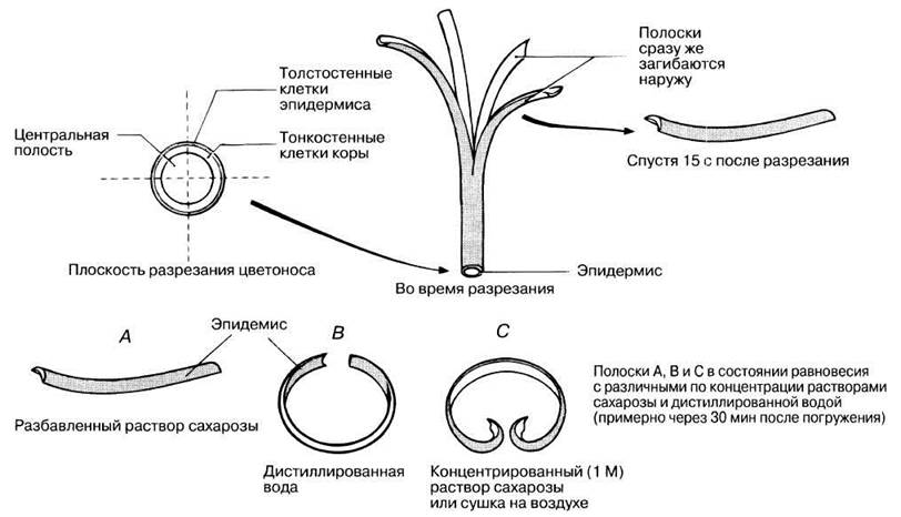
Fig. 13.6. Dandelion scape experiment. Studying The Effect of distilled water and sucrose solutions on the curvature of strips cut from the hollow stem.

13.12. The red pigment in beetroot is located within the cell vacuoles. Based on this, design experiments to investigate the effect of high temperatures and alcohols on the semipermeability of beetroot cell membranes.