Biochemical Engineering Fundamentals, Part 1 - Bailey J., Ollis D. 1989

Transport phenomena in biotechnological systems
Determination of kia' and power consumption of stirred-tank and sparged reactors

In this section, we summarize the results of various Experiments on the study and Methods of determining the volumetric mass transfer coefficient k_ia'. Since a' cannot be directly determined, experimental data are often expressed precisely as the parameter k_ia'. Furthermore, in some cases, this complex parameter accounts for effects due to the significant residence time of small bubbles in highly viscous media. In such cases, the bubbles contain virtually no oxygen and therefore make no contribution to O₂ transfer. For this reason, for example, a' values determined by optical methods may not reflect the actual specific interfacial area of oxygen-containing bubbles.

We have already noted that an increase in the specific power consumption can lead to a decrease in gas bubble size and thus to an increase in the interfacial area. Here, we describe methods for calculating the power consumed by the Reactor using parameters that define the characteristics of sparging and mixing devices. In addition, we will consider a fairly common case of simultaneous agitation by spargers and mechanical stirrers.

Many METHODS FOR STUDYING mass transfer in gas–low-viscosity liquid systems in stirred tank reactors are reviewed by Van 't Riet [9]. The results of A large number of experiments in various reactors using impellers of different designs can be described with an accuracy of ±20–40% by the following equations:

Stirred tank reactor, Water, coalescing system:

Class="center">

Stirred tank reactor, water, non-coalescing system:

Here, u_gs is the superficial gas velocity, equal to the volumetric gas flow rate divided by the product of the reactor cross-section and the gas holdup. Below each equation, the ranges of reactor volume and volumetric energy consumption for which these expressions are valid are indicated.

It should be emphasized that, in accordance with the Basic principles of The Effect of turbulence on mass transfer discussed above, these equations are valid (within the specified accuracy of ±20–40%) for A wide variety of mixing devices (turbine, paddle, propeller, and bar impellers, self-inducing devices) and different numbers of impellers. THE POSITION OF the impeller in the reactor also does not play a significant role, unless its distance from the bottom of the reactor is too small (less than its diameter), which can reduce The rate of power dissipation, or if the impeller is located too close to the surface, which is accompanied by air entrainment and a reduction in power consumption.

Similarly, studies of mass transfer in bubble columns have shown:

Bubble Column, water, coalescing system:

K_la = 0,32(u_gs)^0,7      (8.73)

For a non-coalescing system in a bubble column, no general correlations exist, since the sparger design affects the value of k_la'.

Since determining the power consumption or superficial gas velocity can be difficult, we present several empirical equations of other types as Examples. Thus, for gas transfer in a bubble column, Akita and Yoshida proposed the following equation [12]:

Here, the column diameter d_t is taken into account in the Bond (Bo ≡ gd_t²p_c/σ) and Galileo (Ga ≡ gd_t³/u_l²) numbers. It has been shown that this equation is applicable for d_t ≤ 60 cm (0.6 m) and can be used for d_t > 60 cm if d_t in equation (8.74) is taken as 0.6 m.

Bello et al. proposed the following equation to determine the volumetric mass transfer coefficient k_la in an airlift column [13]:

Here, A_d/А_r is The ratio of the cross-sectional areas of the downcomer and riser Zones of the disperse system, and P/V is the ratio of the power consumed for aeration to the volume. This equation can be used, but it does not account for the fact that mass transfer, gas holdup, and other parameters are not uniform across the different zones of the airlift apparatus.

Any empirical equations have a limited range of applicability. Thus, the strong effect of P/V on k_la' predicted by equation (8.75) does not hold at sufficiently low P/V (P/V < 1), since under such conditions, the dynamics of gas bubbles in the liquid phase are primarily determined by natural convection, i.e., their free rise.

To disperse and subsequently mix the liquid phase, as well as to maintain the upward flow of bubbles and reduce or completely eliminate large bubbles and air pockets, static mixers can be used. To determine mass transfer in such apparatuses, Wang and Fan proposed the following equation [14]:

FIG. 8.6. Mean flow velocities (expressed as fractions of the impeller tip speed of 5.2 ft/s) (1.6 m/s) and water Circulation pattern in a 12-inch (30.5 cm) deep tank at an agitation speed of 200 rpm. (McCabe W. L., Smith J. C., Unit Operations in Chemical Engineering, 3d ed., p. 234. McGraw-Hill, New York, 1976.)

Here, u_g and u_l are the superficial velocities of gas and liquid (in cm/s), respectively.

A potential drawback of any empirical equation is the assumption of uniform energy dissipation and/or a constant value of k_la' in the mixing zone where the parameters underlying the equation were measured, as well as in the reactor under study or design. In this regard, it is useful to consider the Changes in the mean flow velocity experimentally observed in a standard baffled stirred tank reactor. The curves in Fig. 8.6 indicate the circulation flow patterns, while the numbers represent local mean velocities as fractions of the impeller tip speed.

Several studies on bubble columns have shown that the value of k_la' significantly depends on the Location OF THE measurement point within the column volume. Fig. 8.7 shows the results of the experimental Determination of the axial dissolved oxygen distribution in a bubble column and in a three-phase system—a fluidized bed containing 0.1 cm diameter particles. In both cases, there is an inlet zone near the sparger where oxygen transfer rates are relatively high; as the distance from the sparger increases, the oxygen transfer rate drops sharply. This phenomenon is likely due to the transition from bubbles of one size, determined by the sparger parameters, to bubbles of another diameter, which depends on the equilibrium between bubble coalescence and breakage. The values indicated by the symbol □ in Fig. 8.7 were calculated using a mathematical model assuming plug flow of gas through two zones with different volumetric Mass transfer coefficients. It was found that the boundary between the two zones is located approximately 33 cm above the sparger. In another model for a bubble column of a different design, it is assumed that kia' initially decreases (for the first 27.6 cm from the sparger) and then reaches a constant value.

FIG. 8.7. Experimentally determined (1) and mathematically modeled (2) profiles of dissolved oxygen concentration versus distance from the sparger for a bubble column (u_l = 7,5 см/с, u_g= = 28 см/с) (а) and a three-phase fluidized bed containing 0.1 cm diameter particles (u_l = 7,5 см/с, u_g = 20 см/с) (б). The curves show the general trend of the relationships. [Reproduced with permission from: Alvarez-Cuenca M., Nerenberg M. A., in Advances in Biotechnology, vol. 1, p. 477, Moo-Young M. (ed.), Pergamon Press, 1980.]

Certain difficulties can arise during scale-up operations. For instance, the aforementioned inlet zone contributes significantly in small laboratory systems, whereas in tall, large-volume columns, it represents only a minor fraction of the total volume.

We now proceed to the methods for calculating the power required to achieve specified gas input rates in a bubble column and for mechanical agitation. Here, we will discuss only the General Principles of these methods and some equations; a more detailed Treatment of energy losses in equipment components can be found in the literature cited at the end of the chapter. For a bubble column, the power required to compress the gas to a level that ensures sparging at a volumetric flow rate F₀ at pressure р₁ is given by the equation

Here, р₂ is the pressure at the top of the vessel, u₀ is the gas velocity at the sparger orifice, and а is the fraction of gas kinetic energy transferred to the liquid; typically, а is approximately 0.06.

The power consumption for agitating non-aerated liquids depends on the DENSITY AND VISCOSITY of the liquid medium, р_l and μ_l, the impeller rotational speed N_i, and its diameter D_i, as well as the impeller drag coefficient CD_i. The dependence of the latter parameter on the impeller Reynolds number must differ for each flow regime—laminar, transitional, or turbulent. Fig. 8.8, a presents the results of the well-known studies by Rushton, Costich, and Everett on three different impeller designs [26]. These results are presented as the dependence of a dimensionless parameter—the power number Рnо [defined by Equation (8.78)]—on the impeller Reynolds number Re_i:

In the turbulent regime, the power consumption is independent of Re_i, i.e.

Conversely, in laminar flow, these relationships are described by the expressions

FIG. 8.8. a—Power number versus Reynolds number for various impeller designs. [From: Aiba S., Humphrey A. E., Millis N. F., Biochemical Engineering. Academic Press, 1973 (Russian Translation: Moscow, Pishchevaya Promyshlennost, 1975); data adapted from Rushton J. H., Costich E. W., Everett H. J., Power Characteristics of Mixing Impellers, part 2, Chem. Eng. Prog., 46, 467 (1950)] b—Friction factor f for pipe flow versus Reynolds number (z—relative roughness of the pipe surface). [Reproduced with permission from: McCabe W. L., Smith J. C., Unit Operations of Chemical Engineering. McGraw-Hill, New York, 1954; data adapted from: Moody L. F., Trans. ASME, 66, 671 (1944).]

In each specific case, the proportionality constant is determined by the design of the mixing device. The similarity between the curves in Fig. 8.8, a and the plot of the friction factor f versus the Reynolds number for pipe flow is noteworthy. In the latter case, the friction factor is proportional to 1/Re in laminar flow (the power number is also proportional to 1/Re_i), whereas in the turbulent regime, f approaches an almost constant value, which is higher for pipes with a rough inner surface. Similarly, as the impeller geometry becomes less 'smooth', Р_nо for the turbulent regime reaches a higher constant value (Fig. 8.8, a); this situation, however, is complicated by the Influence of the vessel walls and baffles on the determined power consumption Р.

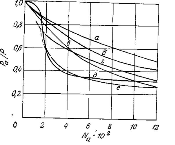
FIG. 8.9. Ratio of power consumption in aerated (Р_а) to non-aerated (Р) reactors as a function of N_a (see text): a—flat-blade turbine impeller (8 blades); b—vaned disk (8 vanes); c—vaned disk (6 vanes); d—vaned disk (16 vanes); e—vaned disk (4 vanes); f—paddle impeller. [Reproduced with permission from: Ohyama Y., Endoh K., Power Characteristics of Gas-Liquid Contacting Mixers, Chem. Eng. Japan, 19, 2 (1955).]

If a stirred reactor is simultaneously aerated, the power consumption for agitation decreases. Fig. 8.9 shows the curves of Р_а/Р (the ratio of power consumption in an aerated reactor to that in a non-aerated reactor) as a function of the dimensionless parameter N_a (aeration number):

Here, F_g is the volumetric gas flow rate.

Except for the most rapidly changing Regions of the respective curves, these relationships can be described by the equation

where m is a coefficient. Michel and Miller proposed another equation, which is also applicable to the turbulent aeration of Non-Newtonian fluids [28]:

Where m' is a coefficient. In equations (8.80) and (8.81), the symbol P denotes the power consumption of the non-aerated reactor, which is calculated using the formulas presented earlier in this chapter.

These equations indicate that at constant N_i and D_i, the power consumption decreases as N_a increases (i.e., with an increase in the air flow rate F_g). This effect is partly due to a decrease in the average density of the agitated dispersed system. At the same time, the mixing efficiency of the system decreases as N_a increases.

In certain bioreactor designs, mixing is achieved using a liquid jet. In this case, the power dissipation can be determined by the following equation [29]:

Where D_j is the jet diameter.