FUNDAMENTALS OF PHYTOCENOLOGY AND PLANT GEOGRAPHY - T. P. Larkina - 2017

SECTION 1. FUNDAMENTALS OF PHYTOCENOLOGY

1.2. Main Parameters of a Phytocenosis

Each phytocenosis is characterized by a set of specific features. Its primary features (or parameters) are as follows: floristic or species composition;

2. vertical stratification (tiering);

3. Abundance;

4. quantitative and qualitative species ratio;

5. frequency (constancy);

6. cover;

7. vitality;

8. aspect.

The Study of a region's vegetation cover begins with a detailed Description of the most typical phytocenosis. To do this, a sample plot is selected and its boundaries are defined within an area that is relatively homogeneous in terms of relief. The plot size depends on the type of plant community. For instance, in a forest, it ranges from 200 to several thousand square meters, whereas in meadow studies, it may vary from 25 to 100 m². Its main parameters are then investigated.

1) Species (floristic) composition is one of the most crucial characteristics of a phytocenosis. It is largely determined by the flora of the given area. The number of species comprising a phytocenosis can vary significantly—from several hundred in a tropical forest to just a few in the tundra. Phytocenoses represented by a single species, which occur extremely rarely in nature, are called monophytocenoses. The number of species per unit area is referred to as the species richness of a phytocenosis.

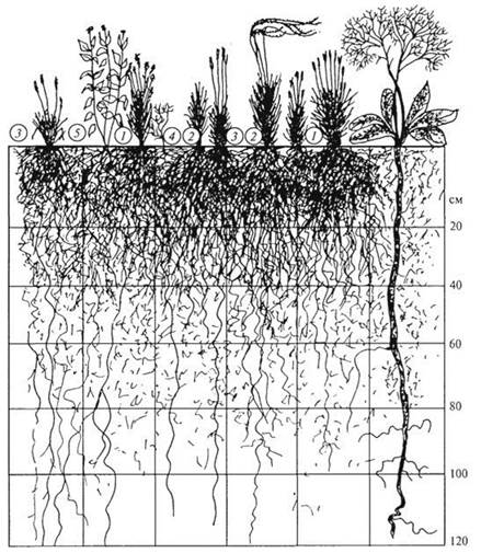
2) Vertical stratification (tiering). In every phytocenosis, plants vary in height, meaning they are spatially segregated. Stratification is determined by the vertical Differentiation of the phytocenosis, the phenological phase of each co-inhabitant, and its requirement for sunlight at any given moment. A distinction is made between above-ground (Figs. 2, 3) and underground (Fig. 4) stratification. Above-ground stratification is particularly distinct in forest phytocenoses (Figs. 3, 5), where it is relatively constant, whereas this parameter is more dynamic in herbaceous communities. Underground stratification refers to the vertical distribution of ROOT systems of different plant species, determined by changes in soil moisture and fertility with depth. This parameter is investigated less frequently in specialized studies.

Class="center">Figure 2. Vertical PROJECTION OF THE herbaceous stand in a steppe meadow in Oryol Oblast

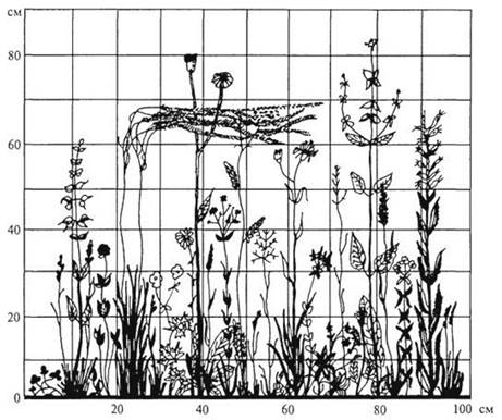
Figure 3. Profile diagram of a tropical forest on the island of Kalimantan; forest strip about 60 m long and 8 m wide, trees over 7 m tall

Figure 4. Underground stratification of a steppe community (Abdurakhmanov, 2007): 1 - crested wheatgrass; 2 - feather grass; 3 - sheep fescue; 4 - wormwood; 5 - sea lavender

Forest phytocenoses can feature 4 to 5 or even more tiers. The uppermost layer, represented by the tallest trees, is always considered the first tier; this is followed by two or three tiers of shorter trees (understory, Secondary Growth), with shrubs forming the next layer (Fig. 5).

Figure 5. Multi-tiered mixed forest

Figure 6. Forb meadow

Figure 7. Feather grass steppe

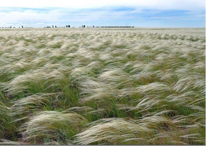
Figure 8. Herbaceous layer of a cowberry pine forest

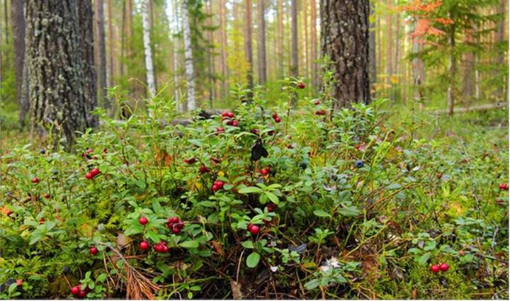
Figure 9. Herbaceous layer of a bilberry pine forest

Figure 10. Mixed pine forest

Figure 11. Lichen pine forest

Figure 12. Pine forest

Figure 13. Forb meadow with blooming buttercups

Figure 14. Sphagnum bog

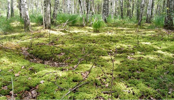
Figure 15. Tundra in summer

Figure 16. Giant sequoia (Sequoiadendron giganteum)

Figure 17. Giant sequoia (Sequoiadendron giganteum)

Figure 18. Eldar pine in Georgia

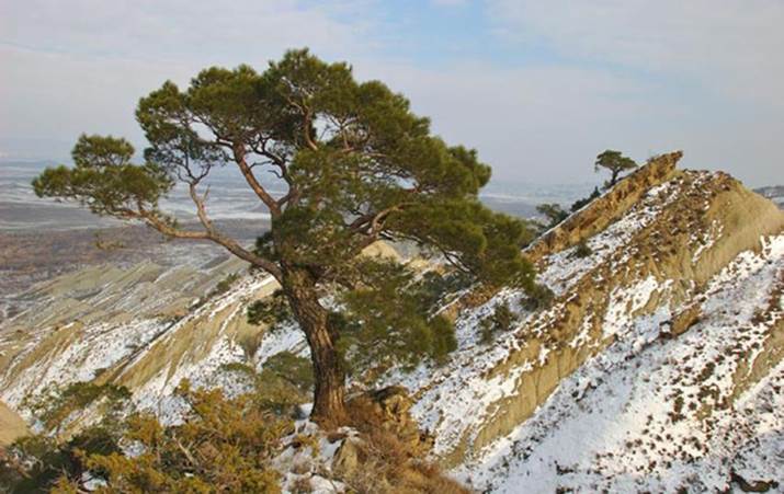
Figure 19. Ginkgo (Ginkgo biloba)

Figure 20. Sweet chestnut (Castanea sativa)

Figure 21. Ginseng (Panax ginseng)

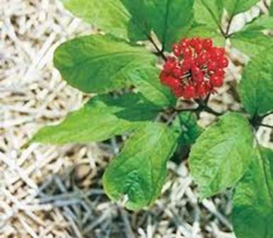
Figure 22. Water shield aquatic plant (Brasenia schreberi)

Figure 23. Marsh Labrador tea (Ledum palustre)

Figure 24. European feather grass (Stipa pennata)

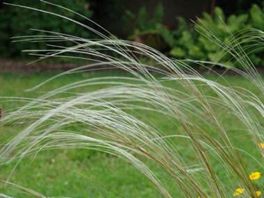
Figure 25. Hairy locoweed (Oxytropis pilosa)

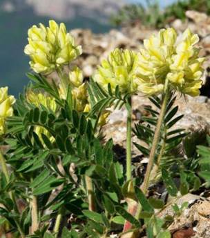
Figure 26. Sheep fescue (Festuca valesiaca)

Figure 27. Dyer's greenweed (Genista tinctoria)

Figure 28. Kungur forest-steppe

Figure 29. Floral regionalization of the globe

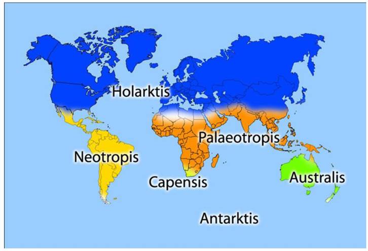
Figure 30. Tulip tree (Liriodendron tulipifera)

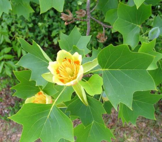
Figure 31. Broadleaf forest

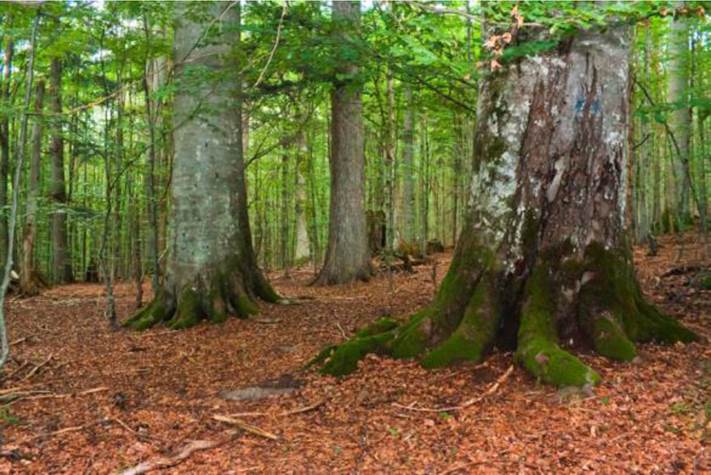
Figure 32. Forest-steppe (I. I. Shishkin, "Rye")

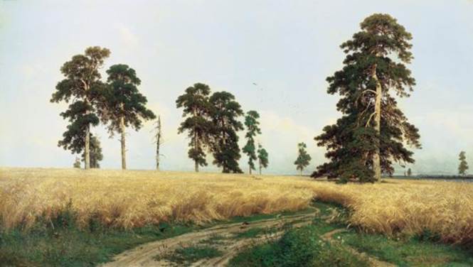
Figure 33. Siberian taiga

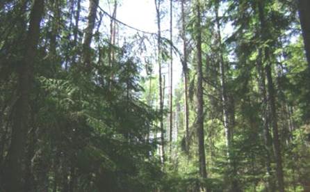
Figure 34. Paleoendemic welwitschia (Welwischia mirabilis)

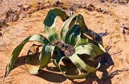
Figure 35. Rafflesia arnoldii

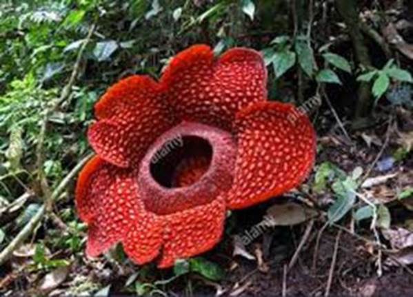
Figure 36. Azorella yarita, a plant typical of the Antarctic floristic kingdom

Figure 37. Botanical-geographical regions of Perm Krai

Herbaceous vegetation forms a separate layer, and the very last layer is represented by the moss cover. When describing meadows, four layers are usually distinguished: the 1st layer, for example, is occupied by the tallest grasses—cocksfoot (Dactylis glomerata), meadow timothy, or plants such as great burnet (Sanguisorba officinalis) and bistort (Bistorta officinalis). The second layer is represented by red clover, and the third by various species of bentgrass. The fourth, lowest layer is occupied by mosses. Phytocenotic layering is a variable indicator, depending on the phenological phase in which a particular species finds itself at a given moment.

3) Abundance (number of individuals). The abundance of individuals of each species within the community's territory is determined primarily by a favorable combination of environmental conditions for that species (soil, moisture, illumination, etc.). When describing a phytocenosis, plant abundance is calculated separately for each species. Phytocenoses differ sharply from one another according to this parameter. Species abundance is determined using several Methods:

a) Visual estimation of species abundance is the most commonly used method. Counting the number of individuals of individual plant species in nature is very difficult; therefore, in practice, rather than determining the exact specific density of individuals of each species, studies of a phytocenosis typically use its qualitative expression—so-called abundance. Its determination is carried out using special scales, in which each grade corresponds to a specific abundance. In Russia, a four-point scale is adopted, in which a score of 4 means that the species receiving this score forms the Background; a score of 3 is given to a plant with abundant distribution; 2 to a plant occurring sporadically alongside others; and a score of 1 is given to a plant that occurs rarely (singly). Essentially, this is a modified and somewhat simplified five-point scale of the Danish botanist Drude: Soc - background plant (f) - score 4; Cop - abundant distribution (ab) - score 3; Sp - occasionally (occas) - score 2; Sol - singly, rarely (r) - score 1. It is evident (Fig. 6) that in this forb meadow, oxeye daisy and cornflower will receive an abundance score of 3, whereas Hair-like feather grass (Fig. 7) will receive an abundance score of 4.

In phytocenological studies across various countries, other scales are also widespread (Table 1).

Table 1. Geobotanical scales

b) The abundance census method by recounting is more labor-intensive, but it makes it possible to precisely determine the number of plants of each species within a sample plot. The size of the plots depends on The Nature of the phytocenosis being studied. Tree vegetation is assessed in plots of 1000 m² or 2000 m². To assess the abundance of shrubs and herbaceous vegetation, the plot size is 100 or 200 m². If more precise results are required when studying meadow vegetation, the plot size is reduced, while their number is increased to 20, distributed pointwise across the entire meadow;

c) The weight method for assessing abundance makes it possible to determine what green biomass a given species or economically-botanical group of interest yields as a percentage of the total biomass of the phytocenosis. This method is important for evaluating the productivity of natural hayfields and pastures. The number of plots is increased to the maximum (up to 20 - 50), and their sizes are reduced to 0.25 m². Plants are harvested "at the root" down to the soil level, then sorted by species or economic-botanical groups, weighed, and average indicators are calculated. Below is a table for determining green biomass in a meadow phytocenosis (Table 2)

Table 2. Weight-based accounting of meadow productivity

4) Quantitative and qualitative ratio of species is an indicator that allows one to establish which species are dominant in the phytocenosis and which are of secondary importance:

a) dominants (dominant species, from Lat. domina - ruling) are those that occur in greater numbers, dominate over other species, create the background, and provide the greatest organic mass; often in each layer of a phytocenosis, one can distinguish its own dominant species (for example, Scots pine in a pine forest (Fig. 12));

b) subdominants occur in smaller numbers than dominants, but make up a significant part of the phytocenosis both visually and in terms of organic mass;

c) accessory species occur rarely, are scattered, and do not shape the plant community. For example, in a bilberry spruce forest (Piceetum myrtilli), spruce is the dominant species, bilberry is the subdominant, and all other species are accessory or even tertiary.

METABOLISM/2.html">THE CONCEPT OF "dominant" is closely related to that of the edifier. An edifier (from Lat. aedificator - builder) is defined as a species that, due to its abundance and productivity, plays a leading role in creating the phytoclimate within a community. These concepts are closely related but not identical: every edifier is always a dominant, but not every dominant (especially a subdominant) is an edifier. For instance, in a forest phytocoenosis, the trees act as edifiers: in a pine forest, it is the pine (Fig. 10); in a birch forest, the birch.

5) Species constancy (presence). Species within phytocoenosis are distributed unevenly. This can be related to both microrelief and the biological CHARACTERISTICS OF THE species. To determine the constancy coefficient in various areas of a herbaceous phytocoenosis, at least 20

sample plots with an area of 0,1 m² are established; in forest phytocoenoses, their area increases to 100 m2 or more, while the number is reduced to 10. Then, the presence or absence of each species in each plot is recorded in a table. Below is a sample table for determining the Raunkiær frequency index in a meadow phytocoenosis (Table 3).

Table 3. Determination of the frequency index

The frequency index is calculated using the formula:

R is the frequency index (Raunkiær frequency),

a is the number of sample plots containing the given species,

n is the total number of plots in the studied phytocoenosis.

6) Vitality. The Development of various species within a phytocoenosis is not uniform. Vitality refers to the capacity of a given species to develop fully or partially under specific environmental conditions. For instance, some species bloom, others produce fruits and seeds, while still others typically reproduce only vegetatively. Vitality is usually denoted by numbers: 3 — the species completes its full developmental cycle; 2 — the species only vegetates normally; 1 — it exhibits only weak vegetation.

7) Canopy cover (projective cover). Along with abundance, projective cover—which essentially represents the projection of aboveground plant parts onto a flat surface (the soil surface)—is of great importance in characterizing a phytocoenosis. This indicator allows us to assess both the overall density of the plant cover and the proportion contributed by its constituent species. Projective cover is expressed as a percentage. In herbaceous communities, cover can be estimated visually by looking vertically downwards, or by using a simple device (Ramensky grid) — a 10x10 cm square grid subdivided into smaller squares, each representing one percent. For tree layers during ground-based surveys, cover is determined visually by assessing canopy closure when viewed vertically from bottom to top. Aerial photography is a more modern and precise method in forest research.

8) Aspect refers to the general appearance, color features, and physiognomy of a phytocoenosis. The aspect is determined by many factors, the primary ones being species composition, the phenological phases of co-occurring plants, and environmental factors. Aspect changes manifest during the alternation of wet and dry or cold and warm seasons. This is most distinct in meadow grass communities, where several aspect-forming species can be observed throughout the growing season — for instance, the mass flowering of buttercups in a meadow (Fig. 13) or the browning of sedges In the second half of summer. Pine forests and spruce forests practically do not change their aspect throughout the year, remaining evergreen. The physiognomy of Sphagnum moss carpets in bogs (Fig. 14) and Lichens on rocks is quite stable.

The change of aspects is determined by their coloration, which depends on the phenological phase of dominant and subdominant species. The aspect (physiognomy) of a phytocoenosis is determined by the phenological phases of dominant and subdominant plants at the time of observation. Aspect shifting is closely linked to Changes in the vertical stratification of co-habitants, as plants typically reach their maximum height during mass flowering. This parameter — aspect dynamics — is of great significance in studying the vegetation of inaccessible high-altitude regions, northern territories, the Arctic coast, and Antarctica using aerial and satellite imagery methods.

9) Phenological observations are an integral part of studying a phytocoenosis, since all its components are subject to constant seasonal changes driven by the succession of their phenological phases. The branch of botany that studies seasonal changes in the plant life cycle is called plant phenology. For every plant, seasonal changes (the transition of phenological phases) occur in a strictly defined order. A woody plant in a temperate climate typically goes through six phenological phases: 1

— vegetation (onset of sap flow, bud Swelling, etc.); 2

— budding (swelling of flower buds); 3 — flowering; 4

— fruiting; 5 — end of the growing season (yellowing of leaves, leaf fall, etc.); 6 — dormancy period.

Annual grasses go through nine phenological phases: 1 — seedlings (regrowth); 2 — appearance of the third leaf; 3 — tillering; 4 — stem elongation (jointing); 5 — heading (booting/ear emergence); 6 — flowering; 7 — grain formation; 8 — grain filling (milky and dough ripening stages); 9 — grain ripening (waxy and full maturity). For herbaceous perennials from different families, the phenological phases differ slightly. For red clover, for example, 5 phases are distinguished: 1 — seedlings; 2 — inflorescence formation; 3 — flowering; 4 — browning of flower heads; 5 — seed maturation. In wild strawberries (woodland strawberry), a secondary growth phase is observed after fruiting.

Each phase typically includes subphases: for example, onset of flowering, mass flowering, and end of flowering. Phenological observations are essential because they contribute to the rational management of natural meadows, hayfields, and pastures. The green mass of meadow vegetation harvested at the beginning of flowering has an increased vitamin content and a reduced fiber content, whereas the harvesting of medicinal plants is carried out strictly according to phenological phases, as these determine the concentration of BIOLOGICALLY ACTIVE SUBSTANCES in the plants.