Genetics - A. V. Sivolob 2008

Formal Genetics: Patterns of Trait Inheritance
Deviations from Mendelian Ratios
Determination of Deviation: The χ² Test

Before examining the Causes and Mechanisms of deviations, in each specific case one should answer whether such a deviation from the expected Mendelian trait distribution actually occurs. After all, the lack of correspondence between the expected and real phenotypic ratios can simply be caused by random fluctuations. Let us illustrate this with a simple example of tossing a coin and landing on heads or tails. Obviously, the probability of landing on heads or tails is 1/2, meaning the expected ratio of outcomes is 1 : 1. Specifically, in 10 tosses, there should be approximately 5 heads and 5 tails. The key word in the previous sentence is "approximately"—the greater the number of tosses, the closer the result will be to the expected one. Due to random fluctuations, one typically observes (as is easy to verify) ratios like 3 heads and 7 tails, or 7 heads and 3 tails (and 7 : 3 = 2.333:1, which differs significantly from the theoretically expected ratio).

Thus, random fluctuations can lead to differences between theoretically expected segregations and those observed in an experiment. The larger the Sample size, the smaller such deviations will be. If experimental data differ from theoretically expected values solely due to random fluctuations, the null hypothesis is said to be supported. Otherwise, another explanation for the observed segregations must be proposed, and consequently, a different hypothesis.

To evaluate the null hypothesis in mathematical statistics, the χ² test is used. The χ² value quantitatively reflects the deviation from the expected distribution, taking into account the sample size:

Class="center">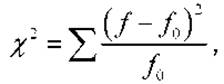

where f is the number of individuals with phenotypes of a certain class in the sample, f_o is the expected number, and the summation sign indicates summing over all phenotypic classes (number n). Suppose, for example, that in a cross of pea plants with yellow and green seeds (Fig. 3.1), the second generation yielded 70 plants with yellow seeds and 30 with green seeds (n = 2). The null hypothesis assumes a 3 : 1 ratio, meaning the expected counts are 75 and 25, respectively. Applying the given formula yields

An important characteristic is also the number of degrees of freedom. Among all phenotypic classes, the probability of occurrence of one class is uniquely determined by the probabilities of the remaining classes, meaning the number of degrees of freedom is m = n - 1. In our example, the number of phenotypic classes is n = 2, and the number of degrees of freedom is m = 1: for a given sample, the number of individuals in one class automatically determines the number of individuals in the other class. It is important to account for the number of degrees of freedom because as this value increases, the probability of random deviation from expected values also increases.

After determining the number of degrees of freedom, it is necessary to interpret the χ² value in terms of the probability (1 - p) that the deviations from the expected distribution are statistically significant (non-random)—in fact, this is precisely the task most frequently facing a researcher. The value of p depends on the χ² value and the number of degrees of freedom; p is usually determined using special tables or graphs. Fig. 3.3 graphically presents the tabular dependence of p on χ² for various values of the number of degrees of freedom. If, for example, a vertical line is drawn from the point 1.333 on the abscissa to its intersection with the curve for m = 1, it can be estimated that in our example p ≈ 0.27.

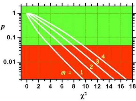
Fig. 3.3. Dependence of probability p on χ² for four values of the number of degrees of freedom m.

The green area corresponds to p > 0.05, and the red area to p < 0.05

The obtained p-value is compared with a certain significance level α, which sets the acceptable probability for the given case of erroneously rejecting a true null hypothesis: if p > α, the null hypothesis is accepted; if p < α, it is rejected, and the observed deviations are deemed statistically significant. Typically, biological research employs α = 0.05. That is, if p < 0.05, then with a probability > 0.95 (the so-called confidence coefficient 1 - α), the observed deviations are considered statistically significant; for all other p-values, the null hypothesis is accepted. Thus, in our example, the null hypothesis is supported. In the previous simple coin-tossing example (also with one degree of freedom), with seven heads and three tails, χ² = 1.6 and p ≈ 0.2—the null hypothesis (the validity of which no one doubts in this case) is likewise supported.

Table 3.2. Values of χ² for two p-values depending on the number of degrees of freedom

In practice, to test the null hypothesis, the calculated χ² value is compared with the critical value corresponding to p = α (Fig. 3.3, Table 3.2). The null hypothesis is accepted if χ² is less than the critical value, and rejected otherwise.