BIOLOGY Volume 2 - A Guide to General Biology - 2004

11. QUANTITATIVE ECOLOGY

11.4. Synecological Study

A synecological study involves examining the abiotic and biotic components associated with a natural community (the biotic component of an ecosystem) found within a specific geographical area (or ecosystem), such as an oak woodland or a rocky shore, where multiple PLANT AND ANIMAL species may live and various habitats (ecotopes) may exist. Such a study requires the following baseline data: 1) a sketch map and, if possible, vertical profiles of the area and ecotopes; 2) identification of the resident species and an estimation of the population size for each; 3) quantitative assessment (and measurement, where possible) of the parameters characterizing the abiotic habitat conditions.

The overarching goal of such a study is to describe, both qualitatively and quantitatively, the interrelationships among plant and animal populations in a given area, as well as their relationships with edaphic, topographic, and climatic factors, where feasible. Once this information has been gathered, researchers can strive to understand what determines the presence, Abundance, and distribution of specific organisms, and to what extent—that is, to outline the food web and, wherever possible, ecological pyramids (of numbers, biomass, and energy).

11.4.1. Mapping the Area

Plane-table surveying

The simple method outlined below is primarily suitable for small areas, such as a clearing or a pond, but it can also be applied to larger tracts, up to an entire rocky bay or even an estuary.

1. Having roughly selected the area for study, lay out a tape measure along one of its sides. This will serve as the baseline AY (Fig. 11.17).

Class="center">

Fig. 11.17. One method for mapping key site details, such as the contours of a small, irregularly shaped pond.

2. From this baseline, measure perpendicular distances to chosen natural landmarks or ranging poles in the field that will define the boundary of the study zone. Record these measurements (for points 1–16).

3. Transfer all these lines (AY and the perpendiculars to points 1–16) to graph paper at an appropriate scale.

4. Using points 1–16 on the graph paper, sketch in the BOUNDARIES OF THE study zone by hand.

5. If the area is relatively small, divide the baseline AY into equal segments and stretch ropes across their boundaries, perpendicular to the baseline. Repeat this Procedure along the far-left transect AF, using it as a second baseline. This will yield a grid like the one shown in Fig. 11.18. Transfer this grid to the sketch map and label the resulting sectors with alphanumeric codes (A1, B2, C3, etc.).

Fig. 11.18. Map of the survey area divided into coordinate sectors (A1–E5, etc.) using a rope grid. The grid ensures more precise designation of study plots during subsequent work.

6. Mark on the sketch map the locations of areas that clearly differ in Structure and vegetation type.

7. Using a quadrat frame, a Levy altimeter, or a rope grid—depending on The Nature of the site—systematically survey the area, say from left to right, noting the species present and the abundance or frequency of their individuals.

8. If the area is very large and a qualitative-quantitative description is required, you can use belt transects crossing the area at regular intervals perpendicular to the observed zonation, combined with random quadrats corresponding to so-called stations (with precise coordinates). If no obvious zonation is apparent, you must rely solely on the random quadrat (station) method. Direct Quantitative determination of abiotic environmental parameters (in the field or in the lab on collected samples) should be carried out as frequently as possible.

Profiling the vertical relief

In certain locations, the distribution of organisms depends on elevation (hypsometric factor). This factor is particularly important on the seashore, for instance, as it determines the duration of immersion and exposure for different zones during the tidal cycle. In such cases, it is necessary to construct a vertical profile showing the altitudinal distribution of various PARTS OF THE survey area along a transect running from its lowest to its highest point. The elevation of each point (station) is determined using a theodolite. Over short distances, a homemade sighting device mounted on a stand of precisely measured length, combined with a leveling staff, can be used for this survey (Fig. 11.19). Let us examine the procedure using the intertidal zone as an example.

Fig. 11.19. A simple homemade device for leveling relative heights, used in conjunction with a graduated staff. The stand of the device is plumbed vertically so that the sighting tube is oriented precisely horizontally. The observer looks through it at the graduated staff held by a partner and notes which mark aligns with the crosshairs.

1. Mount the sighting tube at a convenient, precisely measured stand height (h₁) for observations, for example, at a height of 1.5 m.

2. Set up a linear transect between the low-Water (at ebb tide) and high-water (at full tide) marks.

3. Position the instrument along this transect, for example at the high-water mark, and place the leveling rod at a measured distance (x) further down the slope. These will be stations A and B. While conducting the survey, walk along one side of the transect to avoid trampling the organisms living along it, which will be sampled later.

4. Level the sighting device precisely (using a plumb line) and determine the point on the rod it is "aiming" at (have the person holding the rod point to it when you look through the tube). This will be the height h₂. Record this value. The elevation difference between stations A and B will be h₂ - h₁.

5. Move the instrument to station B, and move the rod further down to a distance x₁. This will be station C. Repeat steps (3) and (4) to determine the next height h₃ (Fig. 11.20).

Fig. 11.20. Profile surveying on a rocky shore: measuring heights and horizontal distances along a straight line between stations located above the low-water mark.

6. Continue the survey to obtain heights h₄, h₅, etc., and distances x₂, x₃, etc. (stations D, E, etc.) down to the low-water mark. Record all distances and elevation changes as shown in Table 11.6. Calculate the elevations of the stations above the low-water mark.

Table 11.6. Horizontal and vertical distances for stations A–K on a rocky shore (Northumberland, 1968)

7. Plot these data to scale on graph paper, drawing a vertical profile showing the positions of all stations (Fig. 11.21).

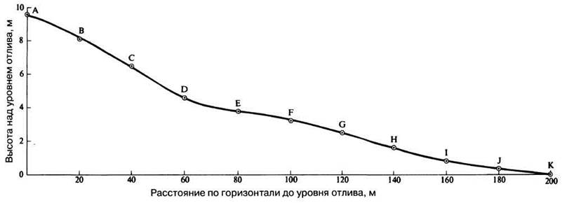
Fig. 11.21. Data from Table 11.6 plotted as a rocky shore profile showing the locations of sampling stations A–J. Note that the unit length on the abscissa is 10 m, while on the ordinate it is 1 m. As a result, the profile shape in this figure is artificially distorted, but it still effectively illustrates the distribution of gently sloping and steep sections of the intertidal zone.